10 Supplements/appendix

10.1 Supplement: Fortune Cookie Wisdom

Here are some broad lessons that I hope you take away from this module, And that will help you throughout… I will come back to these.

It may seem like we have the answers, but this is only where we have asked the questions very carefully

But sometimes ignorance is bliss.

Examples: Sunk-cost fallacy, gains to trade/comparative advantage, opportunity cost, free-riding/prisoners’ dilemma, double-marginalization,‘raise price to raise profit’, etc.

I’ve had many discussions about these things with my non-economist wife. Some of them make her more sanguine and content; other stress her out.

We are building models based on very precisely defined assumptions, usually assuming things like a ‘single representative consumer’. These models are seductive and very helpful for clearly conveying insights.

However, when it comes to applying these things to the real world, or testing these models, be careful; people may differ and they may change and they may have multiple motives.

10.2 Supplement: market imperfections can suggest business opportunities

A major theme in Economics is: Markets work well but not perfectly. Imperfections in existing markets \(\rightarrow\) opportunities.

Audio/slide presentations

HERE, starting at 44:20, ending about 51:30.

Or starting at 31:00 HERE:

Although we are not focusing on ‘market failure’ in this module (BEEM101, 2020)…

I don’t want you to go away thinking that economists believe, ‘markets solve everything, markets yield the best of all possible worlds’. The simplest models do aim to show the conditions under which this holds, but that is not a good characterization of most economic work. Most economists recognize the existence of market failures, and I believe that most recognize the usefulness of government intervention in many cases. Difference of opinion mainly arise over the prevalence of these market failures, and the extent to which government can do a good job of fixing them, or ends up making things worse.

I’m not telling you what you need to believe, I just don’t want you to have a false impression of mainstream Economics.

I also believe that these apparent imperfections or market failures actually can lead to opportunities to create value and profit. Things that were once market failures might be solved by technology or new frameworks.

Here are some possible examples.

Imperfection: Inefficient monopoly markups for information goods

\(\rightarrow\) ‘All you can eat’ \(\rightarrow\) Spotify, Netflix, Kindle Unlimited

When people who value certain goods which could be shared with them at no cost, are nonetheless priced out of this market, this represents an inefficiency. The only price per unit that will lead to the efficient amount of consumption Would here be a zero price. However, firms and content providers cannot stay in business with zero prices. On the other hand, if they can get a good signal of what people would be willing to pay for ‘all-you-can-eat’ And then charges this to them as a subscription fee, Those consumers who subscribe will then consume the efficient amount. This represents an example of a two-part tariff, a form of price discrimination which may actually increase welfare. We will learn more about price discrimination later.

Free-riding on public goods

\(\rightarrow\) Disneyworld, resorts

We will see that markets will not provide the efficient amount of certain goods that are non-rival and non-excludable. However (as for the information goods case), 4 large enough territory some of these things like fireworks can essentially be made excludable. Disney World has fireworks every night, and they own such a large property that they can exclude people from coming anywhere near where the fireworks are being shown, so it would be hard to free ride. They then charge an admission fee to ‘be inside of Disney World’ and then they want to make the experience of being inside Disney World as nice as possible, so they produce a great deal of what would otherwise be considered public goods.

Imperfection: Lack of information about ‘experience goods’, lack of trust in one-shot-interactions

\(\rightarrow\) Uber, AirBnb

Another potential market failure comes from Asymmetric information (we won’t cover this in detail); consumers may not know the quality of a product until after they have purchased it. In some cases, this means no one may be able to sell a certain product because consumers will not trust its quality, the so-called ‘lemons problem’ or ‘adverse selection’. Reputation systems, particular those developed on Internet sites like Uber and Air B&B, can help reduce this problem and create new markets (and profit for themselves).

Shyness and fear of ‘losing face’

\(\rightarrow\) Tinder

Perhaps two people want to work together, or socialize or romance each other. However they may both be afraid of the consequences of being rejected. Even though both would like to be ‘partnered’, neither will make an overture to the other because the risks seem too high.

A third-party intermediary, man or machine, could be set up to only share information about ‘Mutual matches’. Once again, this will create fruitful transactions and the intermediary may be also be able to profit.

If you’re interested, see my research on this here, presentation slides here, my research page is here.

Asymmetric information, adverse selection

\(\rightarrow\) NHS, ‘Obamacare’

This one is a government intervention, obviously. However, private corporations are very deeply involved in these markets and healthcare systems; even in the UK, where healthcare Is perhaps more Directly provided by the government than anywhere else in the world, there are private providers like BUPA.

Insurance markets can fail because of a problem of ‘adverse selection’. A given set of insurance policies will tend to be more attractive to those people who envision their at more risk; in the context of health insurance, more likely to become sick and require hospitalization. Because of this, insurance companies will need to charge rates that reflect risks for the less healthy population. Because of this, healthier people may be ‘priced out of the market’, i.e., prefer to not obtain insurance. This may be inefficient because Even these healthy people may be ‘risk-averse’, and would benefit from purchasing ‘actuarially fair insurance’ (We will define these terms later).

There is a strong case to be made that a mandate to purchase insurance (or system of fines and subsidies) can improve overall outcomes in these situations. This is the logic behind several healthcare systems and proposals, including the USA Affordable Care Act passed under the Obama administration, and some aspects of the Netherlands’ system as well.

Note: Firms themselves do not typically use markets: if we look inside the firm and see all sorts of mechanisms to correct or circumvent internal markets. Understanding when and why firms do this, and the trade-offs involved, can help you be a better manager. For example, when should you ‘outsource’ and when should you keep a task in house? When should you offer employees very strong incentives and when should you just tell them what to do?

Major theme: Markets work well but not perfectly. Imperfections in existing markets \(\rightarrow\) opportunities.

I don’t want you to go away thinking that economists believe, ‘markets solve everything, markets yield the best of all possible worlds’. The simplest models do aim to show the conditions under which this holds, but that is not a good characterization of most economic work. Most economists recognize the existence of market failures, and I believe that most recognize the usefulness of government intervention in many cases. Difference of opinion mainly arise over the prevalence of these market failures, and the extent to which government can do a good job of fixing them, or ends up making things worse.

I’m not telling you what you need to believe, I just don’t want you to have a false impression of mainstream Economics.

As I also mentioned, these apparent imperfections or market failures actually can lead to opportunities to create value and profit. Things that were once market failures might be solved by technology or new frameworks.

Here are some possible examples.

Imperfection: Inefficient monopoly markups for information goods

\(\rightarrow\) ‘All you can eat’ \(\rightarrow\) Spotify, Netflix, Kindle Unlimited

When people who value certain goods which could be shared with them at no cost, are nonetheless priced out of this market, this represents an inefficiency. The only price per unit that will lead to the efficient amount of consumption Would here be a zero price. However, firms and content providers cannot stay in business with zero prices. On the other hand, if they can get a good signal of what people would be willing to pay for ‘all-you-can-eat’ And then charges this to them as a subscription fee, Those consumers who subscribe will then consume the efficient amount. This represents an example of a two-part tariff, a form of price discrimination which may actually increase welfare. We will learn more about price discrimination later.

Free-riding on public goods

\(\rightarrow\) Disneyworld, resorts

We will see that markets will not provide the efficient amount of certain goods that are non-rival and non-excludable. However (as for the information goods case), 4 large enough territory some of these things like fireworks can essentially be made excludable. Disney World has fireworks every night, and they own such a large property that they can exclude people from coming anywhere near where the fireworks are being shown, so it would be hard to free ride. They then charge an admission fee to ‘be inside of Disney World’ and then they want to make the experience of being inside Disney World as nice as possible, so they produce a great deal of what would otherwise be considered public goods.

Imperfection: Lack of information about ‘experience goods’, lack of trust in one-shot-interactions

\(\rightarrow\) Uber, AirBnb

Another potential market failure comes from Asymmetric information (we won’t cover this in detail); consumers may not know the quality of a product until after they have purchased it. In some cases, this means no one may be able to sell a certain product because consumers will not trust its quality, the so-called ‘lemons problem’ or ‘adverse selection’. Reputation systems, particular those developed on Internet sites like Uber and Air B&B, can help reduce this problem and create new markets (and profit for themselves).

Shyness and fear of ‘losing face’

\(\rightarrow\) Tinder

Perhaps two people want to work together, or socialize or romance each other. However they may both be afraid of the consequences of being rejected. Even though both would like to be ‘partnered’, neither will make an overture to the other because the risks seem too high.

A third-party intermediary, man or machine, could be set up to only share information about ‘Mutual matches’. Once again, this will create fruitful transactions and the intermediary may be also be able to profit.

If you’re interested, see my research on this here, presentation slides here, my research page is here.

Asymmetric information, adverse selection

\(\rightarrow\) NHS, ‘Obamacare’

This one is a government intervention, obviously. However, private corporations are very deeply involved in these markets and healthcare systems; even in the UK, where healthcare Is perhaps more Directly provided by the government than anywhere else in the world, there are private providers like BUPA.

Insurance markets can fail because of a problem of ‘adverse selection’. A given set of insurance policies will tend to be more attractive to those people who envision their at more risk; in the context of health insurance, more likely to become sick and require hospitalization. Because of this, insurance companies will need to charge rates that reflect risks for the less healthy population. Because of this, healthier people may be ‘priced out of the market’, i.e., prefer to not obtain insurance. This may be inefficient because Even these healthy people may be ‘risk-averse’, and would benefit from purchasing ‘actuarially fair insurance’ (We will define these terms later).

There is a strong case to be made that a mandate to purchase insurance (or system of fines and subsidies) can improve overall outcomes in these situations. This is the logic behind several healthcare systems and proposals, including the USA Affordable Care Act passed under the Obama administration, and some aspects of the Netherlands’ system as well.

Note: Firms themselves do not typically use markets: if we look inside the firm and see all sorts of mechanisms to correct or circumvent internal markets. Understanding when and why firms do this, and the trade-offs involved, can help you be a better manager. For example, when should you ‘outsource’ and when should you keep a task in house? When should you offer employees very strong incentives and when should you just tell them what to do?

10.3 Supplement: is Microeconomics applicable to nature… outside of humans?

Studies of honeybees have found that they generally do not gather all of the nectar in a particular flower before moving on.

Why not?

What key features do modern human economies have that ‘animal economies’ don’t have? Largely: trade, prices, specialisation, free choice vs instinct.

The economics of trade may also apply to the natural world in certain ways.

Above, we see the working of ant-aphid symbiosis, a form of mutualism. Relevant to the ‘conditions necessary for trade to occur’? The ants ‘farm’ the aphids, who secrete nice substances. In return the ants protect the aphids and only sometimes eat them.

10.4 Supplement: Empirical research

See an earlier lecture video below, starting at about 1:37:30.

Empirical research: Uses evidence from the real world, i.e., observation, to answer questions (rather than introspection and theory)

Econometrics: The ‘science’ of using data to answer economic questions; Uses statistical tools and often economic theory

Micro-data: Data where the unit of observation is an individual, household, firm, etc.; (Contrasts from macro-data, data on aggregates like GDP, inflation, etc.)

See, e.g.,

‘Macro-data’

This is contrasted from ‘Macro-data’ which is aggregated/averaged in some way (e.g., at the country-level or industry-level)

E.g.,

Econometrics often has a different focus and different methodology than ‘regular statistics’. Econometrics has taken on a larger role in economics over the past 40 years, because of greater data availability and computing power. Most published papers in Economics now involve some econometric (i.e., empirical) analysis.

Throughout the module we will come back to the discussion of empirical work, testing, measuring, and estimating.

10.4.1 Empirical meta-example

Suppose we are trying to estimate the market demand curve; suppose we hypothesize that this demand curve is a linear function. (I.e., suppose we assume that quantity demanded is a linear function of price).

\[Q_d = a-bp\]

Suppose we know that price is changing because of cost changes, shifts in supply curve, or the firm experimenting.

Otherwise the problem is poorly identified, as demand and supply will jointly determine price

We observe price and quantity data for a period where ceteris paribus is reasonable, such as the data below⁴

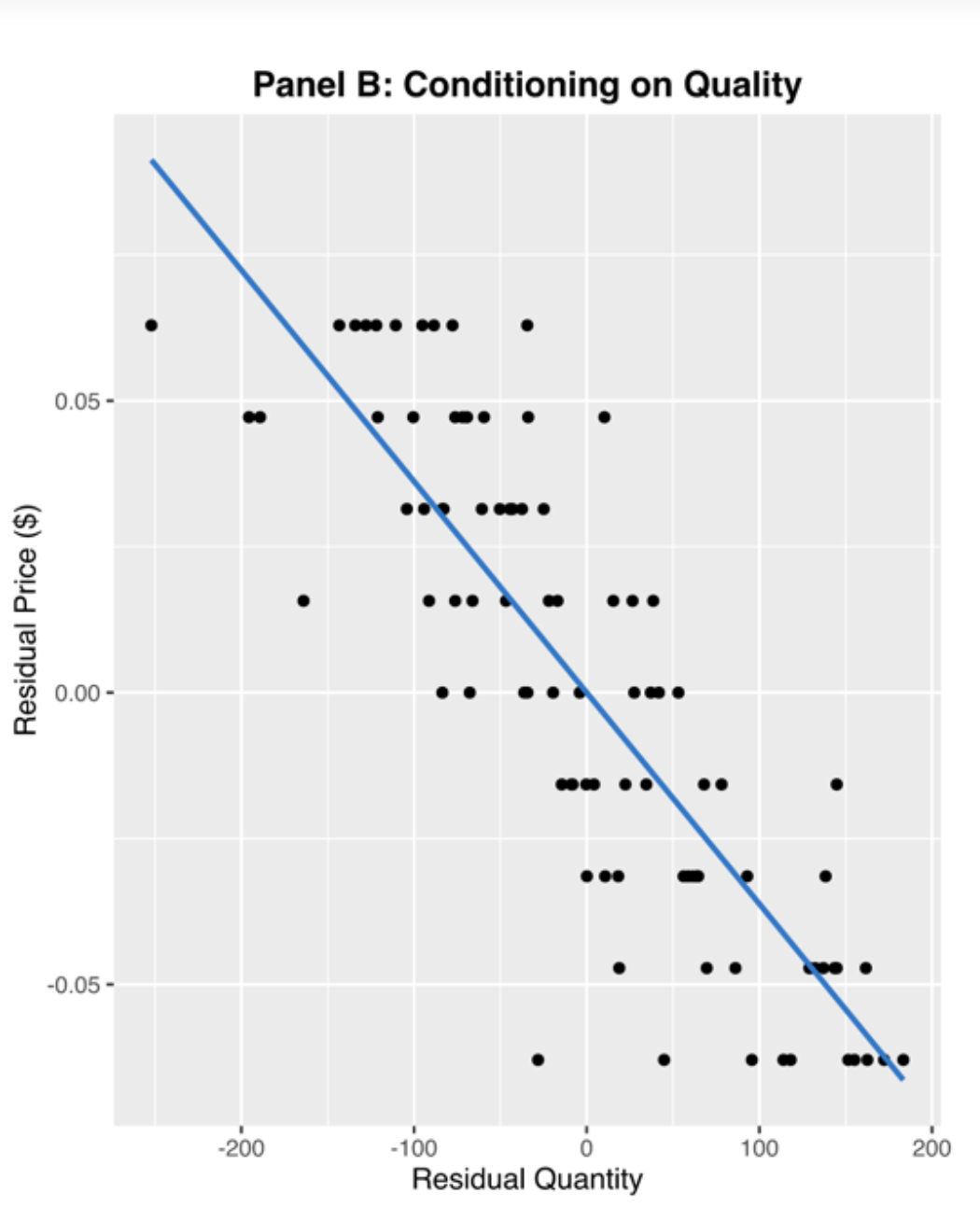
We try to fit the ‘best’ line through these points (minimizing the distances between the line and the points, or minimizing the ‘error’ of this predicted quantity). We estimate the demand curve’s slope and intercept. We can use this to make inferences.

This line will never fit exactly, because of unobserved differences, nonlinear demand, measurement error, randomness in behaviour.

But this fitted line is only meaningful if we are observing shifts in the supply curve and not the demand curve! (Can you explain why?)

Some more in-depth discussions of estimating demand and/or supply curves:

From Econometric online text, Shalabh, IIT Kanpur http://home.iitk.ac.in/~shalab/econometrics/Chapter17-Econometrics-SimultaneousEquationsModels.pdf)

Notes on estimating these models in R using 2sls

10.4.2 Ceteris paribus

All [most] economic theories employ the assumption that ‘other things are held constant.’

In above data/figure, demand may differ between weeks/stores, weather may change, etc.
‘the points may lie on several different demand curves, and attempting to force them into a single curve would be a mistake.’
- \(\rightarrow\) We would like to carefully ‘control’ for other observable factors

May also use flexible functions permitting heterogeneity – differing slopes.

We can never control for everything or know ‘true’ functional form. Sadly, all empirical work involves imperfect compromises.

But happily there are ways to test and validate the estimates, e.g., see how well they predict future outcomes.

10.4.3 Exogenous and endogenous variables

Suppose a model of supply and demand with ‘exogenous shifters’:

\(W\) is an external or exogenous variable that increases the quantity demanded at any price
- E.g., the amount of a windfall tax rebate, boosting net income
\(Z\) is an exogenous variable that makes production more costly, increasing the price firms require to supply a particular quantity
- E.g., the level of the minimum wage, or e.g., energy prices

We can then write the supply and demand model as: \[Q=-P+W\] \[P=Q+Z\]

P and Q are the endogenous variables
- Don’t ask ‘how does P change in Q?’
W and Z are the exogenous variables
- If we know W and Z we can solve for the equilibrium Q and P
- Can observe how this equilibrium responds to shifts in Q and P

10.4.4 More advanced material on causal inference

-The mixtape, Scott Cunningham pp 18-22, and more

Autor, MIT ‘Microeconomic theory and public policy’, lecture 2

We now consider the very very fundamental building blocks behind the (in)famous ‘neoclassical economics model.’ Accept these ’axioms and nearly everything flows from it!

10.5 Supplement: Gains to voluntary trade

Indifference curves and ‘convex combinations’ give us insight into why people trade with one another. It may seem obvious but historically and even in the present, some people see trade as a zero-sum game, with a winner and a loser. But if this were the case, why would both parties sometimes consent to making such a trade?

Considering [figure to be added] , an individual is ok with giving up soda for hamburgers or vice/versa along her indifference curve. A trade that put her above the IC makes her ‘strictly’ better off.

So consider if one individual had allocation D and another allocation A, and they had the same preferences.

What trade could they make to make each of them better off?

Note that a straight line between these two points describes the combinations of ‘shares of bundles A and D adding up to 1’ (e.g., 1/3 of D and 2/3 of A) or ‘trading a fraction of bundle D for the same fraction of bundle A, and vice versa.’

E.g., a 50-50 split of each bundle yields, in this case, (6+2)/2 = 4 hamburgers and (2+6)/2=4 soft drinks.

Note that the line between two bundles depicts all ‘convex combinations’ of these \(\alpha\) of D and \(1-\alpha\) of A, where \(\alpha \in (0,1)\).

In normal-speak, a partial share of each bundle.

We can see that with the same DMRS for both, trades along this line make both better off; the points they would trade to depends on their bargaining power. They might also trade in a way that puts one below this line but still above the original indifference curve.

For an alternative depiction using indifference curves, where preference differ but allocations are the same, see the online text HERE under ‘Case in Point: Preferences Prevail in P.O.W. Camps’

However, trade between two individuals is better illustrated using an “Edgeworth box”, see, e.g., the explanation HERE on economicsdiscussion.net.

10.6 Supplement: Quasiconcavity (of utility function/preferences)

This is the ‘preferred assumption’ which resembles convexity, but has several advantages as a concept. For example, it doesn’t require differentiable preferences, and its properties are not affected by monotonic transformations of utility functions. This is the concept that you might be taught in a PhD module. I think it may also have some value in understanding optimization problems in general, which is an important part of research and industry and finance, I believe.

More formal concept: (strictly) convex preferences \(\Leftrightarrow\) (strictly) ‘quasiconcave’ utility function, allowing ‘n goods’:

This essentially means that for a ‘convex combination’ of any two bundles \(\mathbf{A}=(X_A,Y_A)\) and \(\mathbf{D}=(X_D,Y_D)\)

\[U(\alpha\mathbf{A}+(1-\alpha)\mathbf{D})\geq\alpha U(\mathbf{A}) + (1-\alpha)U(\mathbf{D})\]

where \(0<\alpha<1\).

Note the switch to a ‘weak inequality’ here for quasiconcavity, strict for ‘strict quasiconcavity’*)

E.g. (with two goods),

\[U(\alpha X_A + (1-\alpha)X_D,\alpha Y_A + (1-\alpha)Y_D) \geq \]

\[\alpha(U((X_A,Y_A)) + (1-\alpha)(U(X_D,Y_D)\]

where \(0<\alpha<1\).

We also describe it as having ‘a convex upper contour set’: the set of all bundles strictly preferred to a particular bundle is a ‘convex set’, implying it contains all convex combinations of elements of this set.

One reason economists like this ‘quasiconcavity’ is because it rules out the ‘false summits’, the local, but not global optima, so we only need to use the first-order conditions to find the optima.

But is this ‘looking under the streetlight to find our keys’ or is it truly without loss of generality?

Without quasiconcavity there may also be no demand function only a demand correspondence: at a given price and income there may be more than one optimising choice!

Can you illustrate this with ‘double-humped’ indifference curves?

Gravelle and Reese appendix, on constrained optimisation (unfold)

A local maximum is always a global maximum if (a) the objective function is quasiconcave, and (b) the feasible set is convex.

It will also tend to rule out ‘sharp jumps’ in response to price changes, so we can look smoothly at ‘comparitive statics.’

Note that ‘quasiconcavity’ does not require differentiability.

Furthermore, unlike properties like ‘diminishing marginal rates of substitution’ this is preserved under a ‘monotonic transformation’ (stretching). This means it is called an ‘ordinal property’. Essentially, quasiconcave utility functions yields indifference curves that are ‘convex to the origin’.

All relevant properties of utility functions are unchanged by such monotonic transformations, including the MRS. This is well-illustrated in Autor’s reading (Lecture 3, pp 11-14)

10.7 Supplement: Constrained optimization (with many goods), Lagrangian method

The constrained problem is equivalent to optimising a single unconstrained ‘Lagrangian’ function.

See Autor notes (Lecture 4: Theory of Choice and Individual Demand)

This yields the above optimisation (first-order) conditions
but only where solutions are positive; there are additional non-negativity constraints,
- \(\rightarrow\) should use Kuhn-Tucker ‘complementary slackness’ conditions;
- however, if an unconstrained problem yields a solution that doesn’t violate the contraint, we can ignore it.

Figure 10.1: From Autor notes

We could have derived this without the Lagrangian, simply substituting in the constraint for one good:

\[x=\frac{I-yp_y- ....}{p_x}\] … subtracting the expense on all other goods.

And then solving this unconstrained problem. Taking the derivative of the solved optimum this with respect to the income term \(I\) will give us a similar expression as \(\lambda\), expressing the ‘shadow value’… the increase in utility for an increase in income.

The conditions for an optimum can also be written in vector notation as:

\[\nabla U(\mathbf{x^\ast})= \lambda\mathbf{p}\]

The ‘gradient vector’ of the partial derivatives of utility wrt each element of \(x\), evaluated at the optimum will be proportional to the vector of prices.

When two vectors \(\mathbf{A}\) and \(\mathbf{B}\) are in the same direction, i.e., \(\mathbf{A}=c\mathbf{B}\), no matter their length, the planes perpendicular to this vector are the same plane. (And all vectors along those planes are perpendicular to vectors \(\mathbf{A}\) and \(\mathbf{B}\)).

This implies that at optimum ‘the rate of increase in utility is greatest in the direction of the vector tangent to the budget line (plane)’…

Which tells us that the plane tangent to the ‘(multi-dimensional) indifference surface’ at this point is the budget plane.

10.8 Supplement: Primal and dual of demand (max and min), Hicksian demand, Identities, Slutskly equation

10.8.1 Primal and dual – functions and relationships (doctoral prep):

Indirect utility function: the (max) utility you can get as a function of your income and prevailing prices.

\[V(p_x,p_y,I_0)=max_{x,y}U(x,y) \text{ s.t. } p_xx+p_yy\leq I\]

Here this is the max and not the argmax … it’s the actual utility level not the consumption level(s). (The consumption levels are the Marshallian demand.)

We can find by solving for the utility-maximising choices, and then plugging these in to compute the utility from these.

Expenditure function: How much income you need to to get a certain utility given prevailing prices.

\[E(p_x,p_y,U_0)=min(p_xx+p_yy) \text{ s.t. } U(x,y) \geq U_0\]

Min and not argmin … the expenditure amount

Hicksian (compensated) Demand for X: The amount of X I consume in a ‘minimising expenditure’ bundle that yields some level of utility (\(U_0\))

With two goods, x and y, the Hicksian demand for x is the first, ‘x’ element of the below (‘Hicksian demand vector x,y’)

\[h_{x,y}(p_x,p_y,U_0)=arg\min_{x,y} (p_xx+p_yy) \text{ s.t. } U(x,y) \geq U_0\]

Note: These functions are actually used in ‘structural’ estimates of demand used in merger analysis, pricing, litigation consulting, etc.

These are ‘inverses’ of one another.

This is because ‘Maximise utility s.t. a budget constraint’ is sort of equivalent to ‘minimise expenditure s.t. attaining a particular level of utility’

Expenditure and Indirect utility identities

Look:

\[V\Big(p_x,p_y,E(p_x,p_y,U_0)\Big)=U_0\]

‘My utility when I have enough income (expenditure) to give me utility \(U_0\) … is \(U_0\)’

And

\[E\Big(p_x,p_y,V(p_x,p_y,I_0)\Big)=I_0\]

‘The amount I need to spend to get the utility I can achieve with income \(I_0\) is \(I_0\)’

Hicksian (compensated) and Marshallian (regular) identities

\[h_x(p_x,p_y,U_0)=d_x(p_x,p_y,E(p_x,p_y,U_0))\]

’The amount of X I consume that yields \(U_0\) at the lowest cost…

is the amount of X I would consume if I had the income that allowed me to get utility \(U_0\).’

Totally differentiating these equalities allows us to relate the compensated and uncompensated responses to price changes.

The proof of Roy’s identity is rather involved and uses the envelope theorem. However, I always thought I saw some intuition for it, if we rearrange it.

What is the Envelope theorem?

How much does utility decrease when good X becomes more expensive by \(\epsilon\), i.e., what is \(\frac{\partial V}{\partial p_x}\)?

Well, from our initial consumption point we now lose \(d_X \times \epsilon\) in spending power. The marginal deteriment of that to our utility is the same as if we had lost this in income, which hurts us at rate \(\frac{\partial V}{\partial I}\).

But why is it OK to consider this ‘from the initial consumption point’ and not also consider the adjustment to this? I believe that comes from the Envelope theorem.

Intuition for Sheppard’s Lemma is easier. How much more do we need to spend to get the same utility if \(p_x\) rises?

We must spend, at the margin, at a rate equal to our previous consumption of \(x\), \(h_x\). Again, we don’t need to consider the adjustment to the consumption bundle in answering this particular question because of the envelope theorem.

10.9 Intuition from the ‘Slutsky equation’

\[\frac{\partial d_x}{\partial p_x}= \frac{\partial h_x}{\partial p_x} - \frac{\partial d_x}{\partial I}x\]

At the margin, the change in demand for X in response to a change in its price sums:

The compensated change in demand (the first term); the marginal substitution effect
the income effect multiplied by the amount of X consumed
- because a price increase in X reduces ‘remaining income’ proportionally to how much X is consumed

A similar result applies to a change in another good’s price, with similar intuition

10.10 Supplement: options contracts

The content in this section is largely drawn from Nicholson and Snyder, “Intermediate Microeconomics and Its Application”, 2010, Cengage.

Option contract: Financial contract offering the right (but not the obligation) to buy or sell an asset over a specified period (at a certain price).

Attributes of options:

Specification of transaction: what is bought/sold, how many units maximum, at what price, etc
Period the option may be exercised (from when until when)
Price of the option

Price of options determined by

Expected value of underlying transaction (e.g., for a call option, expected future share price minus strike price)
Variability of the value of the transaction

Option G (a ‘call option’): Right to buy Google share at £500 (£500 ‘strike price’) in December 2020

Worth more the higher the current share price
If \(P_{google}< £500\) currently, then option G is worth more the higher the expected variability in \(P_{google}\)
- Variability can only help the option-holder:
- price increase helps her
- if price falls below £ 500, she doesn’t need to exercise the option

If you didn’t read this you probably would have guessed the opposite. Common sense does not get you everywhere, and definitely not a good mark on exams. I particularly want you to understand those results that are not common sense.

Duration: the longer the better – a longer duration brings a greater chance that the price will rise above strike price (£500)

Note that the results for ‘right to sell = call options’ are similar, just replace the words ‘buy’ with ‘sell’ and reverse the directions (‘rise’ with ’fall), etc.

Classic economist’s argument: you should ‘bet against yourself’ to minimise risk; but this might give you bad incentives to perform. See column about this HERE … “Hedging your bets in hard times”]