5 (Monopoly) Firms’ optimization and pricing, price-discrimination
I plan to add a great deal of content here.
University of Exeter students: You can find a simple video presentation of many of these concepts from my 2018 lecture below:
LINK to 2018 monopoly/PD lectures: less technical, uses graphical slides
Readings:
Textbook reading
O-R chapter 7 (you can skip the discussion of monopolists that maximise something other than profit)
Consult McAfee and Lewis Chapter 15: Monopoly on the ‘Lerner index’ (or ‘Lerner Markup Rule’). Note: the pdf version of this text is easier to read than the html version.
Notes on O-R chapter:
We will focus on the (standard) profit-maximisation goal, although their discussion of other goals is interesting.
They define consumer and producer surplus here to give a brief treatment of the deadweight loss of monopoly.
They also have a very interesting treatment of the two main types of price discrimination; ‘Implicit discrimination’ foreshadows asymmetric information and agency problems.
There are various names of each of these … I am familiar with “second degree = self-selection” and “third degree or ‘explicit segmentation’”. They call the latter ’Implicit discrimination.
Alternative textbook treatments (unfold):
The notes in this book may draw from some of these alternate texts
- NS: 11.2-11.4
- QMC: Appendix A.1 - Monopoly - the vanilla version
Price discrimination in the media and public debate
Some interesting content to bring these concepts alive
This podcast contains many mis-statements; can you identify them?
Some of my own non-technical writing on price discrimination:
- Article: Should we help companies tailor prices to your wage packet?
- With accompanying worked examples
- Somewhat more advanced: ‘The Government May Want to Encourage Price Discrimination by Income’ Linked here
- Teaching discussion; insightful: (Marsden and Sibly 2011)
Material from data science and industry pricing practice
I want to add more here
See “Marketing” chapter in Business analytics with R (Note, this needs some clarification)
5.1 Why study the monopoly?
A monopoly is a single firm operating in a market without competition.
Although this is an extreme situation (the opposite extreme to ‘perfect competition’), we focus on this because:
- The mathematics of the quantity/pricing choices are easy to interpret, and relevant to other environments.
E.g., the optimization is equivalent to the case of ‘monopolistic competition’, which is sometimes argued to be the most realistic benchmark framework. In ‘monopolistic competition’, each firm has a somewhat differentiated product (or ‘location’) and faces a downward sloping demand for its own product. However, with monopolistic competition, unlike under monopoly, as more firms selling related products enter, each firm’s profit dissipates to zero.
It provides a simple example of the “deadweight” welfare loss from firms with market power reducing their supply in order to keep up prices.
We can most simply percent models of price discrimination and segmentation, which is a highly relevant business practice (and may face similar concerns in other competitive environments like monopolistic competition)
Monopolies (or near-monopolies) certainly do exist and have always existed in some industries … And perhaps these are growing even more important (consider the “big 4 tech firms”)
5.2 Monopoly profit-maximisation: simple (undergraduate-level) take:
As noted, a monopoly is a single firm operating in a market without competition.
Such a firm may gain an Economic Profit *.
A monopoly situation can only be sustained by some barriers to entry, discussed below.
A monopoly firm, like all firms, will set it’s quantity \(Q\) to maximize it’s profits \(\pi(Q) \equiv QP(Q)-C(Q)\) where \(P(Q)\) is the inverse demand (the maximum price that can be charged if a firm wants to sell quantity \(Q\)), and \(C(Q)\) is the cost of producing \(Q\).
Under standard simple conditions (discussed below), if the monopoly can only charge a single price, this leads to the monopoly maximising it’s profit by producing \(Q\) such that \(MR(Q) = MC(Q)\) (assuming \(P>AC\)).
This is because under these simple conditions, we simply need to take the ‘first order condition’ … i.e., to find the profit-maximising quantity \[argmax_{Q} \Big(QP(Q)-C(Q)\Big),\] we simply find the unique point where the slope in \(Q\) (the derivative) is zero, so \[P(Q)+QP'(Q) - C'(Q) = 0,\] i.e., \[P(Q)+QP'(Q) = C'(Q)\], i.e., again, \(MR(Q) = MC(Q)\).
Marginal revenue is the rate at which revenue \(QP(Q)\) changes in quantity, which is thus \(P(Q)+QP'(Q)\).
For a small increase in \(Q\):
- The rectangle of revenue increases proportionally to the current price,
- but it decreases at rate \(P'(Q)\) as price must decrease to sell the next unit, and this price decrease reduces revenue in proportion to the current quantity \(Q\). For my money, this example offers the most intuitive example of the product rule for derivatives.
Intuition: the ‘volume’ benefit of increasing \(Q\) is countered by
- a greater cost (producing more always costs more) and
- the need to reduce price (on all units) to get people to buy it.
For a linear demand curve the marginal revenue will have a slope of twice of the inverse demand curve, and the same intercept (see computation below). See HERE for a very simple and clear depiction of monopoly profit maximization with a linear demand curve (and only a bit of oversimplification.)
Suppose \(Q = \alpha - \frac{1}{\beta} P\), so \(P = \alpha\beta - \beta Q\)
Then revenue is \(PQ = \alpha\beta Q - \beta Q^2\) so \(MR = \alpha\beta - 2\beta Q\), as noted, twice the slope of the inverse demand curve
5.2.1 Graphically: Monopoly profit-max
Marginal cost, demand, marginal revenue, and quantity of a monopoly producer
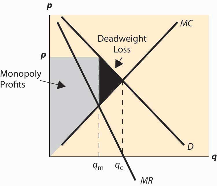
Image source: McDL
Recall that a firm’s revenue is Price \(\times\) Quantity. This is depicted as a rectangle corresponding to a specific point on the demand curve facing the firm.
The firm’s profit is this revenue less average cost.
MR tells you how the ‘revenue rectangle’ will increase (or decrease) with another unit. MC tells you the cost of this additional unit.
This is depicted in the figures below:
Image source: Wikimedia commons
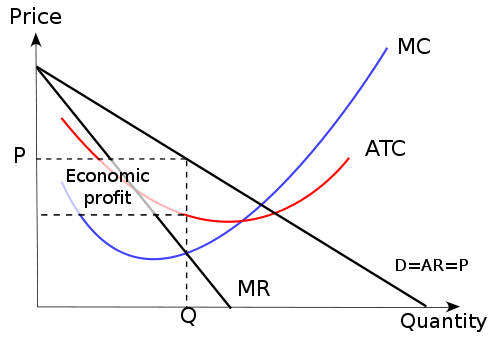
Figure 5.1: Monopoly pricing and profits
Be careful here:
… to see the price charged you need to ‘project up’ to the demand curve NOT the MR curve.
Again, remember that revenue is \(P^*Q^*\) but costs at \(Q^*\) are \(Q^* \times AC\)
so profit is \((P^*-AC)Q^*\).
5.2.2 ‘There is no supply curve for a monopoly!’
A ‘Supply curve’: maps from p to q (and usually vice-versa) for a firm or industry. This is not affected by demand, only by the costs and number of firms.
In contrast:
A monopoly chooses price (thus also choosing quantity it can sell) where \(MR(q)=mc(q)\).
- But \(MR(q)\) depends on the demand curve slope/curvature at \(q\),
- so if the demand curve changes it will affect the supply/pricing decision!
5.3 Monopolistic market, profit-maximization: O-R formal depiction and advanced insights
O-R formally define a monopolistic market. Their definition and approach is unusual because:
Note that they are defining the ‘primitives’ of such a market in a way that allows one to apply rigorous math proofs and (potentially) define an ‘equilibrium’.
They incorporate, from the beginning, a demand function \(q_i(p_i)\) for each ‘segment’ \(i\) … allowing for the possibility of price discrimination (something which we will focus on).
They let the producer have a ‘preference’ (\(\succsim\)), which may incorporate both profit and quantities sold in each segment. We will not focus on this: we will focus on the standard profit-maximisation goal.
This second point is very interesting, but we’ve no time to address it now.
Monopolistic market
A monopolistic market \(\langle (q_i)^k_i=1, C, \succsim \rangle\) for a single good has the following components:
They are just specifying the ‘objects defining a monopolistic market’ here; they have not told us what these things are yet.
Note that we are focusing on a producer of a single good; more complex cases could involve multiple goods with production synergies, strategic bundling, etc.
OR continue:
Demand
The function \(q_i\), the demand function in segment \(i\), associates with every price \(p_i\) for segment \(i\) the total amount \(q_i(p_i)\) of the good demanded in that segment.
They note that these demand functions are ‘decreasing’ functions: for higher values of the argument, the output of the function is not higher. In other words, we are considering demand functions that are decreasing, or at least not increasing, in price.*
This rules out the ‘Giffen’ good.
OR:
Producer A single producer, called a monopolist, characterized by a cost function \(C\) that is continuous and convex and satisfies \(C(0) = 0\),
and a preference relation \(\succsim\) over pairs \(((y_1,... , y_k), \pi)\), where \(y_i\) is the quantity sold in segment \(i\) for \(i = 1,..., k\) and \(\pi\) is the producer’s profit
Note that cost increases in output at an increasing rate; this is a fairly restrictive assumption, and it rules out the ‘natural monopoly’ case. They also assume that the cost of producing 0 is 0, which seems natural.
5.3.1 Profit maximization and marginal revenue
O-R Essentially restate the analysis we presented above, however they are slightly more formal, and they consider an interesting wrinkle: marginal revenue need not be decreasing in quantity.
O-R definitions …
Let \(\langle (q_i)^k_i=1, C, \succsim \rangle\) be a uniform-price monopolistic market.
…we refer to ‘uniform pricing’, because here (as above) we are considering only a single price for the market as a whole. We discuss below why price discrimination my not always be possible, for legal or practical reasons.
Define the total demand function \(Q\) by \(Q(p)=\sum_{i=1}^k q_i(p)\)
… simply summing the quantity demanded at a certain price across all segments 1 through k.
O-R Define marginal revenue essentially as above,
\(MR(y) = [P(y)y]' = P(y) + P'(y)y\), where P is the inverse of Q.
giving additional intuition …
If the function P is decreasing, …
(i.e., if the demand curve slopes downwards)
..we have \(MR(y) ≤ P(y)\) for all y. [Because] selling an additional unit of the good increases revenue by approximately \(P(y)\) but also causes a reduction in the price of all \(y\) units sold.
I restate this point because it’s just that important.
They next make an interesting point which I have not seen noted before:
Usually the function MR is assumed to be decreasing, but this property does not follow from the assumptions we have made. The derivative of \(MR\) at \(y\) is \(2P′(y) + P′′(y)y\)
Of course the MR is itself the derivative of the revenue function, so here we are considering the derivative of a derivative. I.e., the derivative of \(P(y) + P'(y)\) with respect to \(Y\) … and thus considering, ’Is the rate at which revenue increases in output decreasing as output increases, so additional units of output add less to revenue than earlier units? This was the case in all the graphs depicted above, but it need not hold in general.
so that if \(P′′(y)\) is positive and large enough, the derivative is positive even if \(P\) is decreasing.
We assumed above that price is decreasing in quantity (only ruling out ‘Giffen goods’). Thus as the quantity increases the benefit of an additional unit of increase in quantity (holding price constant) must be smaller, because you are charging a lower price. This by itself would point to a declining MR.
However, for every increase in quantity the price must fall somewhat, which itself reduces revenue. The necessary marginal drop in price \(P'(y)\) need not be constant, it may be increasing or decreasing, i.e., \(P′′(y)\) may be positive or negative in any region. Thus, it’s possible that for increases in quantity from a larger starting quantity, the necessary reduction in price is relatively much smaller than it was when increasing quantity from a smaller base, leading to a lower loss of revenue than before, and even outweighing the effect in the previous paragraph.
This is illustrated in O-R example 7.1 involving ‘unit demand’ rather than a continuous demand function, depicting three consumers with ‘maximum willingness to pay’ of 10, 6, and 5, respectively:
| y | p | rev(y) | mr(y) |
|---|---|---|---|
| 1 | 10 | 10 | 10 |
| 2 | 6 | 12 | 2 |
| 3 | 5 | 15 | 3 |
Above, we see that increasing the quantity \(y\) from 1 to 2 requires reducing price from £10 to £6, and thus increasing revenue by only £2. However, increasing the quantity from 2 to 3 requires reducing price by only £1 further, and thus increasing revenue by £3. Although the latter price decrease ‘operates on more prior units’ (2 rather than 1), it is a much smaller price decrease (£1 reduction rather than a £4 reduction), outweighing the ‘volume effect’.
Explaining O-R notation for example 7.1 in response to a student question:
Student:
how [did] they ‘derive’ \(MR(y ) = P(y )y − P(y − 1)(y − 1)\), for the indivisible good. I understand how to reach definition 7.3 but am stuck applying it to this example.
Teacher:
Yes – I think you might be misunderstanding the definition or notation.
\(P(.)\) is a function here, the inverse demand. So \(P(y)\) tells me ‘how much can I charge at most, and still sell \(y\) units’.
They define \(MR\) as ‘the increase in revenue when I sell one more unit’.
Sell 0 units – 0 revenue.
Sell 1 unit, can charge at most £10 … so \(P(1)=10\), and \(Revenue(1) = P(1) \times 1 = 10 \times 1=10\)
Sell 2 units, can charge at most 6, so \(P(2) = 6\), and \(Revenue(2) = P(2)\times 2 = 6 \times 2=12\)
Thus, by their definition, \(MR(y) = P(y)y −P(y −1)(y −1)\), we have \(MR(2)=P(2) \times 2 - P(2-1)\times(2-1) = 6 \times 2 - 10 \times 1 = 12-10 = 2\)
(Also \(MR(2) = Revenue(2) - Revenue(1)\)).
The fact that \(MR\) need not be everywhere downward sloping means that the \(MR(y)=MC(y)\) condition for profit maximizing output \(y\) is a necessary condition but not a sufficient condition.*
* This is not a ‘corner solution’ issue: it is not even sufficient for an interior optimum, with a positive output. Furthermore, this is not because of regions of decreasing marginal costs; it is not sufficient even if MC are constant or rising everywhere.
O-R illustrate this point in Figure 7.1. Have a look.
5.3.2 “Lerner markup rule” – an additional insight
From McDL:
We can rearrange the monopoly pricing formula to produce an additional insight.
(Going back to our earlier notation…)
A profit-maximizing monopolist must set \(Q\) (if positive) such that:
\[P(Q)+QP'(Q) = C'(Q).\] Rearrange this to consider the ‘markup over marginal cost’:
\[P(Q) - C'(Q) = -QP'(Q),\] and now as the ‘markup as a fraction of the price charged’, the so-called ‘Lerner Index’:
\[\frac{P(Q) - C'(Q)}{P(Q)} = -\frac{QP'(Q)}{P(Q)}=\frac{1}{\epsilon} ,\]
The right hand side of this is simply the ‘inverse price elasticity’ \(\frac{1}{\epsilon}\).
Derivation:
Take the inverse of the second term
\(\frac{1}{-\frac{QP'(Q)}{P(Q)}}\) \(=-\frac{\frac{1}{Q}{\frac{P'(Q)}{P(Q)}}\) \(=-\frac{\frac{1}{Q}}{\frac{\frac{dP}{dQ}}{P(Q)}}\) \(=-\frac{\frac{dQ}{Q}}{\frac{dP}{P}}\) \(=\epsilon\)
this formula provides a measure of the deviation from competition, and in particular says that the deviation from competition is small when the elasticity of demand is large, and vice versa.
… If demand is very elastic, the effect of monopoly on prices is quite limited. In contrast, if the demand is relatively inelastic, monopolies will increase prices by a large margin.
This is also a formula firms might directly use … if they knew their marginal cost and, more challengingly, if they knew the price elasticity of demand over its entire range. In the real world, firms do sometimes use ‘markup rules’ for pricing.
According to McDL:
This formula is sometimes used to justify a “fixed markup policy,” which means a company adds a constant percentage markup to its products. This is an ill-advised policy not justified by the formula, because the formula suggests a markup which depends on the demand for the product in question and thus not a fixed markup for all products a company produces.
Some more insights from McDL:
Marginal cost will always be at least zero or larger…. Thus, the price-cost margin is no greater than one, and as a result, a monopolist produces in the elastic portion of demand.
DR: Note that I emphasze at great length that a monopolist will never price in the inelastic portion of the demand curve it faces, and I try to give lots of insight into this.
One implication c … if demand is everywhere inelastic (e.g. \(p(q) = q−a\) for \(a>1\)), the optimal monopoly quantity is essentially zero, and in any event would be no more than one molecule of the product.
5.4 Monopolies and ‘allocative inefficiency’
O-R:
Since \(MR(y) < P(y)\) for all \(y\), an implication of Proposition 7.1 [\(MR(y^{\ast})=MC(y^{\ast})\)] is that the price charged by a profit-maximizing producer in a uniform-price monopolistic market is greater than the marginal cost at this output.
This leads to an inefficiency:
the cost of production of another unit of the good is less than the price that some buyers are willing to pay for the good. The monopolist does not produce the extra unit because he takes into account that the price reduction necessary to sell the extra unit will affect all the other units, too, causing his profit to fall.
Recall from your previous studies, the model of ‘perfect competition’:
Free entry and exit \(\rightarrow\) zero long-run economic profit
Many many tiny firms \(\rightarrow\) firms are price takers.
\(\rightarrow\) price = marginal cost, and in the long run \(p=ATC\) and firms produce at \(min(AC)\)
Similar conditions for input markets (e.g., capital and labor).
This, in combination with firms and consumer’s optimizing behavior, and several other assumed conditions (such as diminishing returns to scale) yielded the ‘fundamental welfare theorems’. Under the first welfare theorem, free exchange and markets ‘in equilibrium’ lead to a Pareto-efficient outcome.
These were extreme assumptions; perhaps only a theoretical ideal.
In contrast, firms with market power might maximize their profits by setting \(p>mc\).
A ‘permanent unregulated monopoly firm’ is the opposite extreme: A single firm, No possibility of competing firms entering, and no competitive or legal constraints on price.
There are a variety of market structures we might consider that fall in between the extremes of perfect competition and monopoly. These include ‘oligopoly’ and ‘monopolistic competition’. The field of Industrial Organization focuses on these models of market structure and their implications for pricing, welfare, innovation, and more
5.4.1 The deadweight loss of monopoly: simple discussion
Criticisms of monopoly:
Monopolies produce too little output, the standard ‘deadweight loss triangle’. This leads to allocative inefficiency (i.e., top-level inefficiency, i.e., the wrong mix of goods is being produced; too little of the monopolized good and too much of other goods).
There is a redistribution of wealth from consumers to owners of monopoly.
(But the latter could be counterbalanced by government redistribution; so maybe we shouldn’t consider it a strike against monopoly?)
Compared to perfect competition, a monopoly typically produces less output and charges a higher price
Some of the consumer surplus under perfect competition is transferred to the monopolist.
There is also a deadweight loss under monopoly, as depicted below. This ‘deadweight’ is lost to society— no one gets it. It represents net value that could be generated but is not generated.
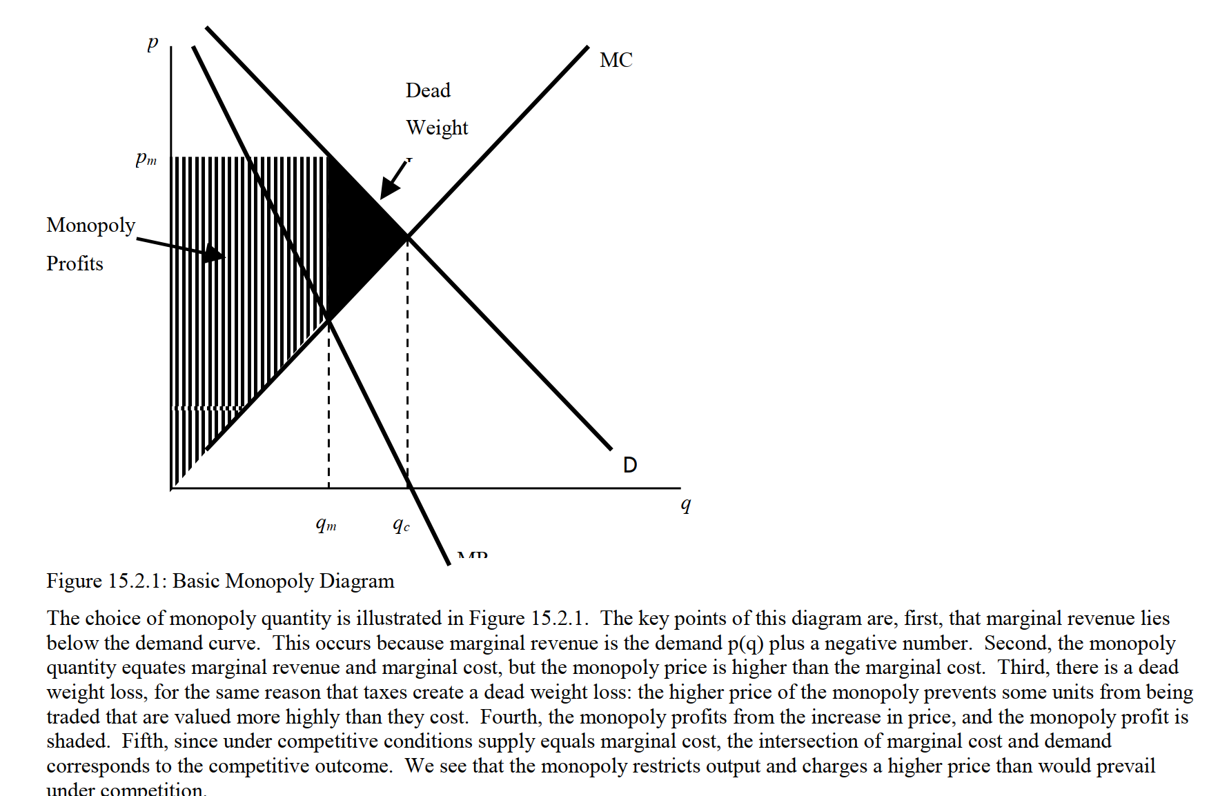
Figure 5.2: Source: McAfee et al.
Be sure you understand and can depict
The difference in monopoly vs perfect competitive quantity
… difference in price
… difference in consumer surplus
… difference in firm profit or producer surplus
Note: The differences mentioned (costs, transfers) refer to the monopoly outcomes relative to perfect competition.
2020 BEEM101 students: For time concerns, I am not going to focus on the measures of the welfare cost or deadweight loss of monopoly, nor on the potential regulatory responses to reduce these costs. These are certainly important for economic policymaking, however. The stereotypical free-market economist is thought to argue that ‘price ceilings are always harmful’; this is not necessarily the case.
Aside: Types of inefficiency; simple definitions
We refer to underprovision of monopoly as a departure from ‘allocative inefficiency’ AKA ’top-level inefficiency’.
Essentially, from the point of view of the entire economy:
- If we could produce more of one good without producing less of any other good (i.e., we are below the ‘production possibility frontier’ (PPF)), perhaps because we are misallocating inputs to different production processes (e.g., capital and labor) … this is called Productive inefficiency
Here ‘goods’ includes all things that people value, including services, environmental amenities, leisure time, etc.
Suppose the economy is producing the combination of goods yielding ‘point Z on the PPF.’ However, suppose that given the combination of goods produced Z, and the distribution of these goods to consumers we could reallocate these. (E.g., have person 1 trade good \(z_1\) to person 2 in exchange for some of good \(z_2\)). Suppose that this reallocation would to make at least one person better off without making anyone worse off (a Pareto imrovement). Then the original point (before any such reallocation) was not Pareto Optimal; it suffered from Exchange inefficiency.
Suppose the economy is producing at ‘Point X on the PPF’ and there is no Exchange inefficiency. However, we are producing the ‘wrong goods’: we could make a Pareto improvement by producing ‘more of one good and less of another’ (and allocating these to consumers). We call this ‘top-level inefficiency’ or ‘allocative inefficiency’. The DWL of monopoly leads to allocative inefficiency: too little of the monopolized good will be produced relative to other goods. (The remaining productive resources will presumably be used towards non-monopolized goods, and these will be relatively over-produced.)
5.4.2 Other potential social costs and benefits of monopoly
Some argue the deadweight loss (DWL) above understates the true harm of monopoly. This is controversial. These arguments include…
‘Secure’ monopolies don’t innovate as much, and spend wastefully (leading to productive inefficiency)?
Monopolies may expend wasteful resources (lobbying, threats, lawsuits…) to preserve barriers to entry
Thus the above monopoly profits may turn into further deadweight losses!
On the other side, some people argue monopolies tend not to persist in the long run, are disciplined by potential entry, and have greater incentives to innovate.
Empirically, the magnitude of the social cost of monopoly is an open question. Estimates range from 0.5% of GDP to 5% of GDP
The double marginalisation problem
Note that if a monopoly firm buys its inputs from a supplier who is also a single-price monopolist, the welfare cost is compounded. There are then ‘two markups’ leading to even more inefficiency.
A simple depiction of the double-marginalisation problem.
Another simple presentation for the case of linear demand can be found HERE on pages 1-6.
This is an argument for letting firms merge with their upstream supplier.
We return to this in the exercises.
5.5 Barriers to entry
If a monopoly firm is earning ‘economic profits’ (profits in excess of the normal risk-adjusted returns to capital), other firms will want to enter the industry. Thus, for the monopoly to persist there must be “barriers to entry”.
What are some ‘Technical barriers to entry’?
What are some ‘Legal barriers to entry’? Explain.
What other barriers might exist?
Technical barriers to entry
1. Increasing returns to scale / Diminishing average cost over a broad range of output \(\rightarrow\) ‘a natural monopoly’
Here multiple firms producing separately are in fact less efficient, as they cannot produce the lowest cost.
2. Special knowledge of a low-cost method of production, or a key resource
* However some argue that there will simply be a limited “rent” derived from this new production process, and it will not constitute a barrier to entry. How would you make such a case?
- A limited market scale with fixed costs and ‘indivisibilities.’ E.g., demand for a particular river crossing may be such that it could support a single ferry operator making a profit, but not two ferry operators. Here there might be a ‘first-mover advantage’.
** Legal barriers to entry**
- Patents and copyrights
- Exclusive franchise or license (granted by government, by another firm, by a university)
- Government support for a dominant firm, discouraging/forbidding others
Other proposed barriers: the threat of ‘predation’
Economists have debated whether “predatory practices” could allow a firm to retain monopoly power. For example, a firm might commit “if any other firms enter we will reduce our prices far below cost.” Perhaps this would scare away other firms from entering.
However, this might not be a “credible threat”; if another firm did enter, the would-be-monopolist might not find it profitable to retaliate in this way. This is an open question; the game theoretic prediction depends on the assumptions made.
… from the 2016 Massachusetts ballot initiative:
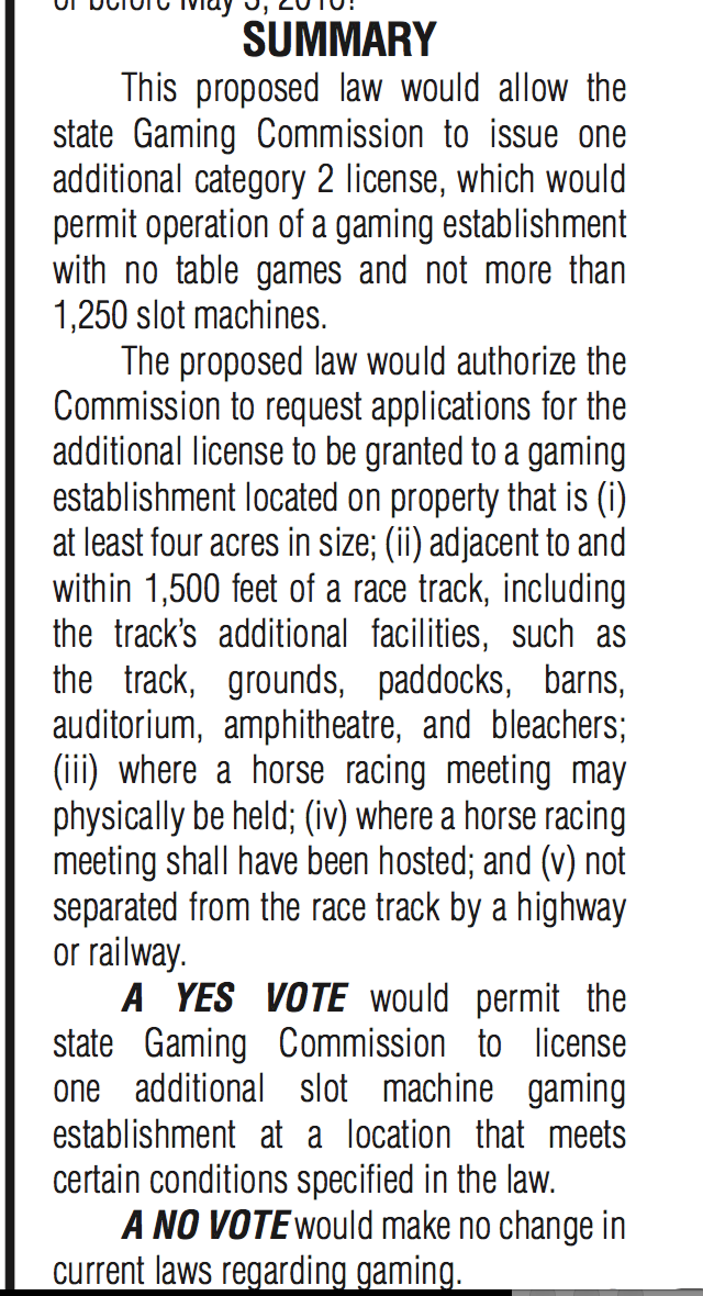
Ballot measure: is this establishing a legal barrier to entry?
5.6 Price discrimination/market segmentation
5.6.1 The basics
Note: This is largely undergraduate material – I plan to update and supplement this soon with more formal material from O-R and elsewhere, and with some applied material from data science and business
- Price Discrimination
The practice of firms offering different prices to different consumers
- Or different prices for slightly different products or quantities,
- where the difference in price does not merely reflect cost difference,
- with the goal of distinguishing consumers’ willingness to pay (WTP).
Note: This includes ‘volume discounts’, or offering an ‘all you can eat’ plan alongside a per-unit plan
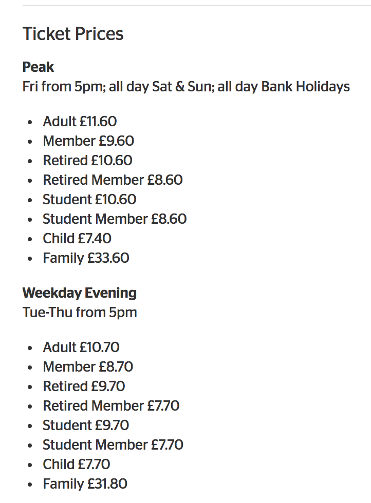
Why such a complicated price list?
Why do firms price discriminate?
It can increase profit… by ‘extracting more surplus’ from consumers
In general, for a monopoly firm, the ability to identify consumers based on their WTP and charge distinct prices will increase profit.
However, it may increase or decrease social (consumer+producer) surplus. Consumer surplus itself may increase or decrease.
Uniform pricing (what we were previously considering… the usual analysis)
Offering a single price for a good for all consumers is known as ‘uniform pricing’.
This does not deal with differences amongst consumers. It may ‘’force the firm to target a particular group’’, such as the wealthy, reducing its total sales.
Under monopoly, uniform pricing leads to a deadweight loss, as we have already seen:
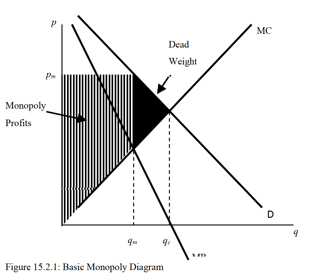
Figure 5.3: Source: McAfee et al.
However, price discrimination holds the potential to increase profit (it will, in general, increase profit). It might also reduce the deadweight loss, i.e., increase total welfare. If price discrimination is ‘Perfect’ then it will boost total welfare, as suggested in the illustration below (see Saylor academy First-Degree Price Discrimination: Personalized Pricing for an interesting discussion, but see margin note.*)
Note: I would say that an auction might lead to outcomes resembling perfect price discrimination, where the seller captures most of the consumers’ valuations. But this is a whole field of study, ‘Auction theory’, which engages the issues of Asymmetric information and Mechanism design (principle/agent models).
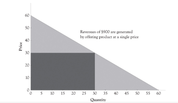
Figure 5.4: Source: Saylor Academy
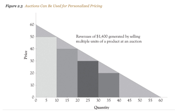
Figure 5.5: Source: Saylor Academy
But if it is not ‘perfect’, price discrimination can reduce (or increase) welfare…
Price discrimination may seem counter-intuitive: ‘how can offering some consumers lower prices increase profit?’
Higher prices increase your profit per unit, but at a higher price you will sell fewer units. The more you charge the less you sell.
Some groups of ‘less keen’ consumers are very sensitive to the price, and they will buy very little at a high price, so a lower price would be more profitable.
Some groups of ‘more keen’ consumers will buy a lot even at a high price. They are less ‘price-sensitive’, so you want to charge them more.
The three types of price discrimination
- Individual-based (First degree; at best ‘perfect’)
Note that ‘targeting a price at each consumer’ may be done on the internet or on a discretionary basis by an individual seller. But this alone does not imply Perfect price discrimination.
‘Perfect’ means the seller exactly predicts and charges each consumer her exact valuation! It’s basically a theoretical ideal.
- Self-selection (Second degree)
For ‘self-selection’ or ‘second-degree price discrimination… we can imagine that the firm doesn’t know each consumer’s valuations. Or, perhaps the firm is not allowed to ’discriminate’ by charging different prices to different people.
Instead, it sells different bundles, quantities or qualities of products to get high and low-value consumers to separate themselves… E.g., first-class seats.
To fully analyse these problems we need to know the techniques of ‘mechanism design under asymmetric information’; we will touch on this later in the module, time permitting, and cover a brief version of it here, following the O-R notes.
There are some interesting results, such as ‘the firm finds it optimal to make the low(er)-valuing type/types’ bundle smaller or lower-quality than would be efficient (called quality or quantity distortion), while the higher-valuing type gets a ‘rent’ (consumer surplus).
- Group-based (Third degree; ‘market separation’)
Here the firm finds something identifiable and inherent about the consumer that is indicative of her likely valuations (and price-sensitivity).
It might be her age, nationality, student-status, or even perhaps her income.
5.7 First-degree and/or ‘perfect’ price discrimination
Is this perfect price discrimination or something else?
The firm can offer each individual a different price for each unit they purchase.
Assuming you know what the consumer is willing to pay, you can make the highest possible profit; that is called ‘perfect’ price discrimination.
- Perfect price discrimination
- Charging each consumer (for each unit) the maximum he or she would be willing to pay, i.e., her valuation
Here the monopolist would extract all the available surplus; no consumer surplus remains.
Because the monopolists extracts all the possible surplus, this is efficient! This holds because the monopolist captures:
\(\max\)(total value of good - cost) \(\rightarrow\) max(CS+PS)
But perfect PD is a rare/impossible extreme: requires mind reading.
A possible close example: a website targets an individualised price to each consumer, based on clues like time-of-day, web clicks, cookie data, IP location. But even this is not really perfect price discrimination: Here, the seller does not really know exactly what the consumer is willing to pay; he is using broad clues.
See Shiller, B. R. (2013, or updated version). First degree price discrimination using big data.
Exeter video: (Monopoly) pricing, ‘perfect’ price discrimination. two part tariffs
For a graphical and algebraic depiction of first, third, and (one version of) second degree price discrimination, please see the video linked HERE from my friend Professor Joon Song.
5.8 Third-degree price discrimination (3dpd) / Market separation
What kind of price discrimination is this? Should it be legal?
Wait: did he just jump from first degree to third-degree price discrimination? Where did second-degree go?
Yes I did. Third degree price discrimination, or ‘market segmentation’ is a much simpler concept than second-degree price discrimination, which involves self-selection. We will return to the latter below.
- Third-degree price discrimination/Market-separation
- The practice of charging different prices to different groups that can be identified
Here, the firm can differentiate groups of consumers or ‘local markets’, not individuals.
Each group has a different willingness to pay on average.
\(\rightarrow\) Offer lower prices to lower-valuing groups, higher prices to higher-valuing groups.
Example: Students and old-age-pensioners may face lower prices for transport, food and other goods; as they have a lower willingness to pay for these
Remember: this is not done out of charity but to boost profits.
Pricing under 3dpd/market separation (calculations/graphical depiction)
Each group or market has it’s own demand \(\rightarrow\) marginal revenue curve
So set an optimising price quantity separately for each group.
E.g., a discount for the elderly, higher price for the middle-aged
Or a lower price in Portugal than in Germany

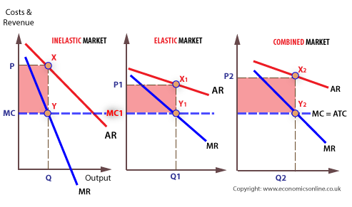
.png)
Consider the above image (from Wikipedia),3
On the left, for the ‘inelastic submarket’ the profit-maximising price is larger than for the ‘elastic submarket’ in the middle.** Note that technically, with linear demand, as shown, the price elasticities vary at every point on the demand curve.
If the submarkets cannot be separated, or the customers in each submarket cannot be distinguished from one another, the firm must charge a single price for the entire ‘industry’ (on the right), which sums the demand curves in each submarket.*
Note that the ‘Industry’ demand curve is kinked at the price where consumers in the elastic submarket begin to buy.
The industry ‘entire market’ price "\(P_m\) will, in general, be in between the optimizing price in the inelastic and elastic markets, so \(P_a > P_m > P_b\) for the above example.
A pretty good numerical example is given in slides 6-8 HERE
Another depiction, adding demand curves (they call it ‘average revenue’):
5.8.1 O-R: Formal treatment of the (monopoly) ‘pricing in multiple markets/segments’ problem
Consider a discriminatory monopolistic market
\[\langle (q_i)^k i=1, C, \succsim \rangle \]
Notation:
\(k\) segments or sub-markets
\(C\) depicts the cost (of production) function
\(\succsim\) represents the monopolist’s preferences; we’ll assume it maximizes profit.
… they assume cost and all segmented demand functions are differentiable.
For each segment \(i\) let \(MR_i\) be the marginal revenue function for \(q_i\), and let MC be the marginal cost function for \(C\).
As they note previously, “this problem cannot be decomposed into \(k\) independent problems because the cost is a function of the total output”.*
* However, if we assume a constant marginal cost, as is often assumed in simplified models, then these problems can be decomposed, and the monopoly will simply set MR=MC in each segment, without needing to consider the other segment.
Because of this, a change in the demand conditions in one segment may impact the optimal price in another segment, through the impact on marginal cost.
E.g., suppose the sole delivery food provider in Exeter is ‘Kangalivery’, which has a separate delivery price for students and non-students. Suppose Kangalivery’s marginal cost of delivering food in Exeter is everywhere increasing. Then if an influx of tourists causes non-student demand to shift outwards, the delivery price for students (as well as nonstudents) is likely to rise, and the quantity provided to students is likely to fall.
If the monopolist’s preferences are profit-maximizing and his optimal output \(y_i{\ast}\) in segment \(i\) is positive, then
\[MR_i(y_i^{\ast}) = MC(\sum_{j=1}^k y_j^{\ast}).\]
O-R offer good intuition for this:
First, the marginal revenues for all segments in which output is positive must be the same since otherwise the producer could increase his profit by moving some production from a segment with a low marginal revenue to one with a high marginal revenue.
Second, if the marginal cost is higher than the common marginal revenue then the producer can [reduce] increase his profit by reducing production, and if the marginal cost is smaller than the common marginal revenue he can increase his profit by increasing production.
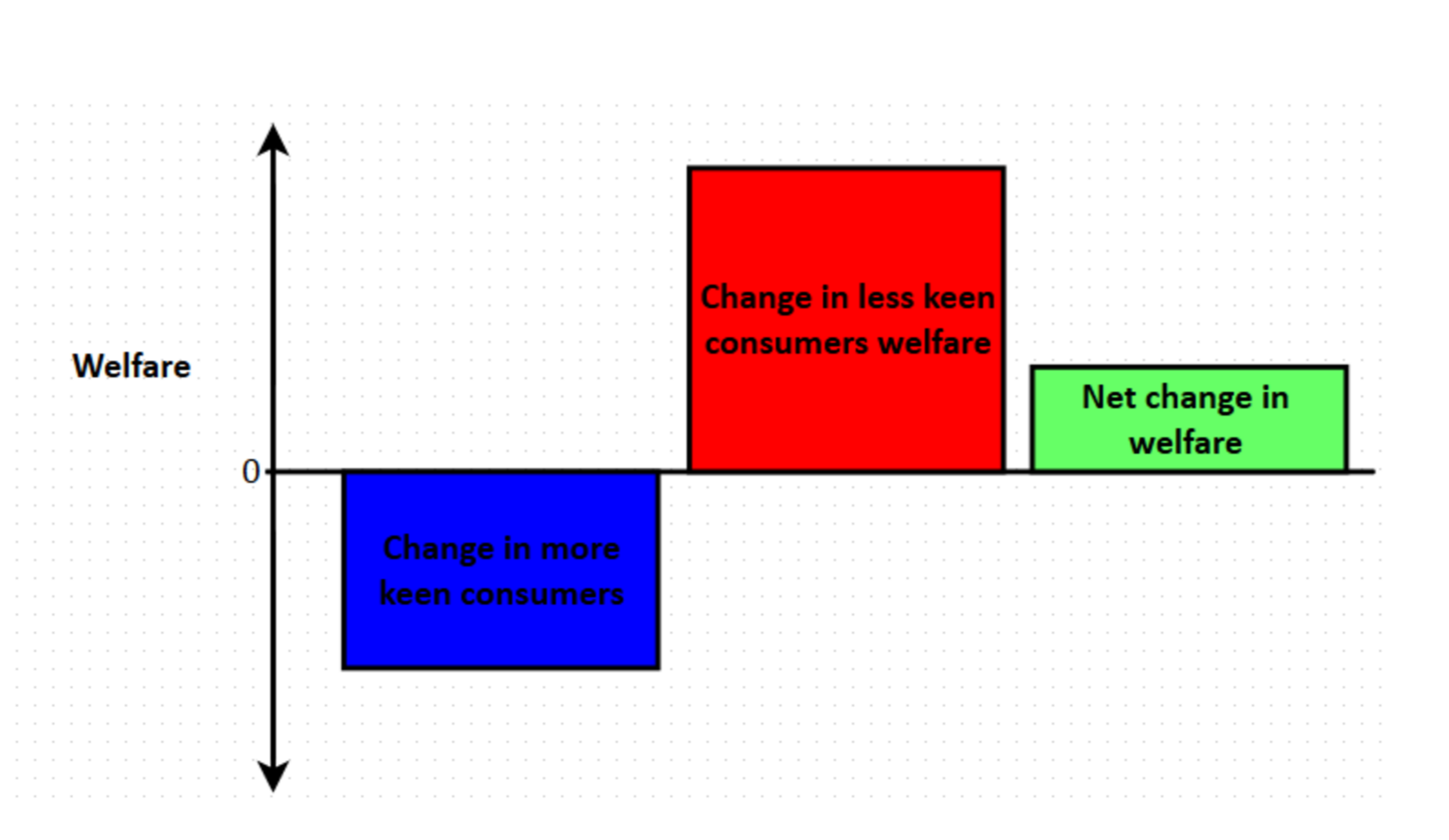
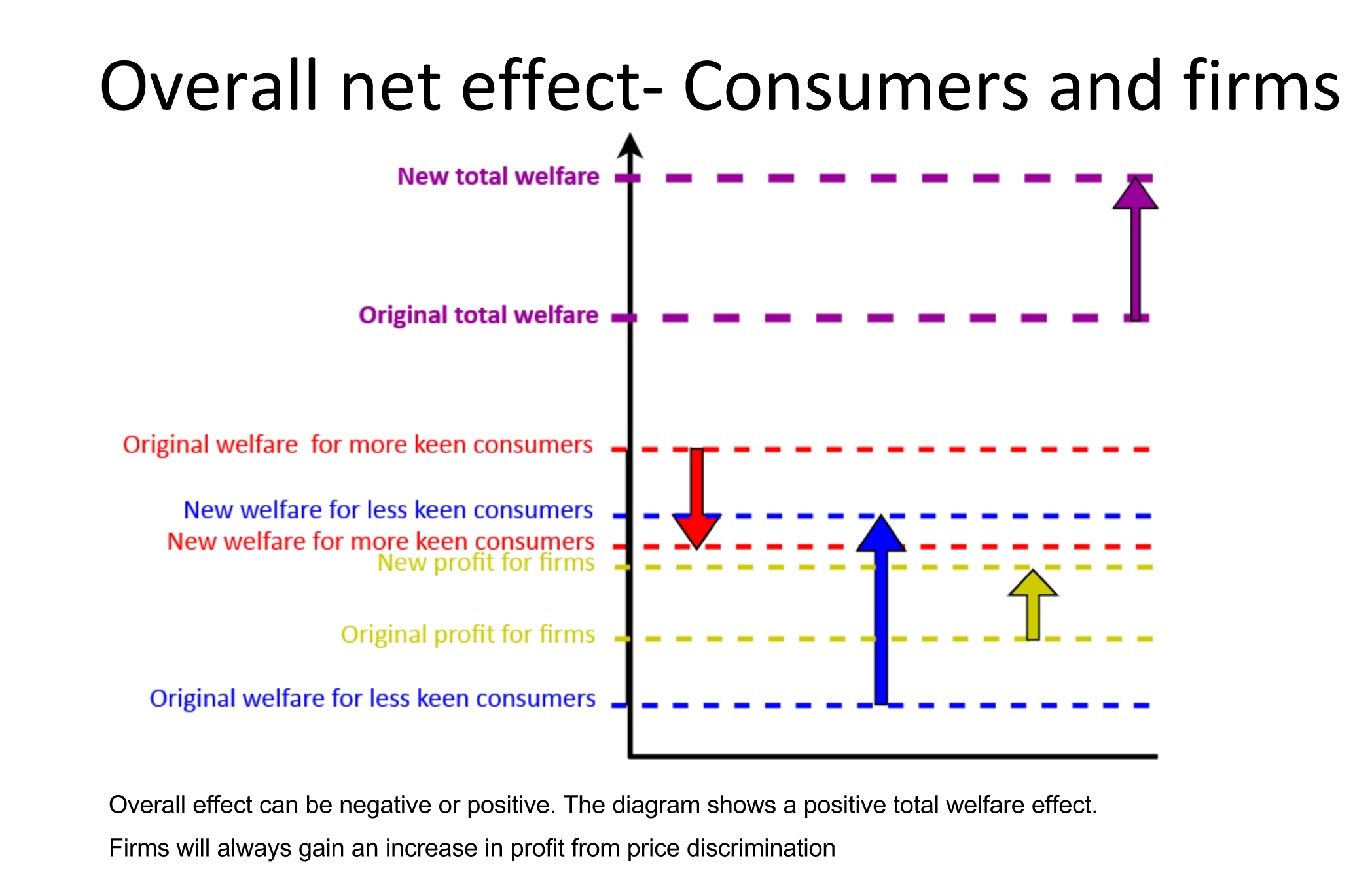
5.9 Who benefits from 3DPD?
Consumers in the identifiable segment with lower wtp face lower prices, thus they benefit
Consumers in the identifiable segment with higher wtp face higher prices, thus they lose
Firms can charge higher prices to high-wtp segment without losing low-wtp segment \(\rightarrow\) increase profit.
Net welfare result: theoretically ambiguous, i.e., ‘it depends’ on several things. This is a nuanced point, but I think you are up to the challenge! This is not covered in most of the textbooks, but I give several explanations below and see references above.
For consumers:
Why is the benefit uncertain?
Exchange efficiency
When groups can be identified as ‘low and high valuation’
the high-valuation groups get charged more, and thus consume less
low-valuation groups get charged less, and consume more
\(\rightarrow\) Exchange efficiency: given what is produced, PD causes it to be consumed by people who value it relatively less!
Top-level efficiency; amount produced
On the other hand, PD could lead more to be produced/consumed (but not necessarily) of the otherwise underproduced ‘monopolised’ good (remember the general DWL of monopoly).
\(\rightarrow\) top-level (allocative) efficiency may increase (or decrease).
E.g., suppose that with a ‘uniform price’ only the wealthy went to a restaurant…
after PD (early-bird discounts, OAP discounts, benefits discounts) the low-income may also dine in the restaurant
\(\rightarrow\) more value is produced
Considering the two effects on efficiency just described … one (Exchange efficiency) is negative and the other (Top-level) may be positive or negative. If the latter is positive (if production increases with PD) the effects trade off one another. Because the ‘Exchange efficiency effect’ is negative, the quantity produced must increase after PD for it to be beneficial. But this quantity increase is a necessary but not a sufficient condition; this effect also must be large enough to outweigh the exchange-efficiency effect.
5.10 Arbitrage … can foil price discrimination
The word ‘foil’ basically means ‘defeat’.
If, e.g., elderly who get discounts could sell the products to the middle-aged…
Then middle-aged would always ask them to do this, never pay high prices
Firm could no longer profit from this
Similar issues with quantity discounts, or ‘web cookie’ personalised pricing
So PD only ‘works’ for goods that are hard to trade, like haircuts…
or where purchases are frequent and low-value, and resale markets are difficult
(The above issues are sometimes referred to as ‘transactions costs’.)
When I ask about the welfare effect of price discrimination, students often mention arbitrage in this discussion. However, the potential for arbitrage doesn’t make price discrimination inefficient, it just makes it ineffectual and makes firms not want to bother doing it.
This yields another mechanism design ‘hidden information’ ‘principal-agent problem’
5.11 ‘Second-degree price discrimination’, i.e., ‘self-selection’, i.e., ‘implicit discrimination’
This section also serves as an ‘applied’ introduction to asymmetric information and principal-agent models (which I cover in more detail in the supplement)
Self-selection and price discrimination is addressed in O-R section 7.4, which I go through below.
However, you might find my ‘semi-parametric’ depiction (following Laffont and Martimort) to be a bit simpler.
Here the firm is unable to differentiate between consumers explicitly. Instead it offers various varieties and bundles. It uses variations in quality or quantity to get consumers to “self-select.”
Some examples:
Quality: Transport- Different classes, Supermarkets- budget products
Quantity: Supermarkets- Larger quantities at lower prices per unit; i.e., ‘nonlinear pricing’
Consider…
Quantity
An 8 ounce cup of coffee for £1.60 vs. 16 ounces for £2.00
- 20 p per oz vs. 12.5p per oz. (with linear pricing there would be the same price of 15p/oz.)
\(\rightarrow\) Result: with 2 prices monopoly can get ‘high value’ consumers to buy/get more in total without losing ‘low-value’ consumers
Quality
The calculations are similar when we consider variations in quality:
An airline doesn’t know whom the high-valuation flyers are (willingness-to-pay, ‘wtp’ for travel itself varies)
But it may know on average that flyers with higher wtp for travel also value comfort more. Thus:
Make second-class seats very uncomfortable, first-class luxurious, and charge more for first-class seats
Can get consumers with higher values for travel and comfort to pay more
…without losing lower-valuing customers
The ‘self-selection’ problem
Train companies must price first and second class such that consumers will self-select.
If first class is too expensive then the high valuing group will not choose first class
If second-class is too cheap, both the high and low groups will choose second class
But if second class is too expensive, the low groups will not buy a ticket.
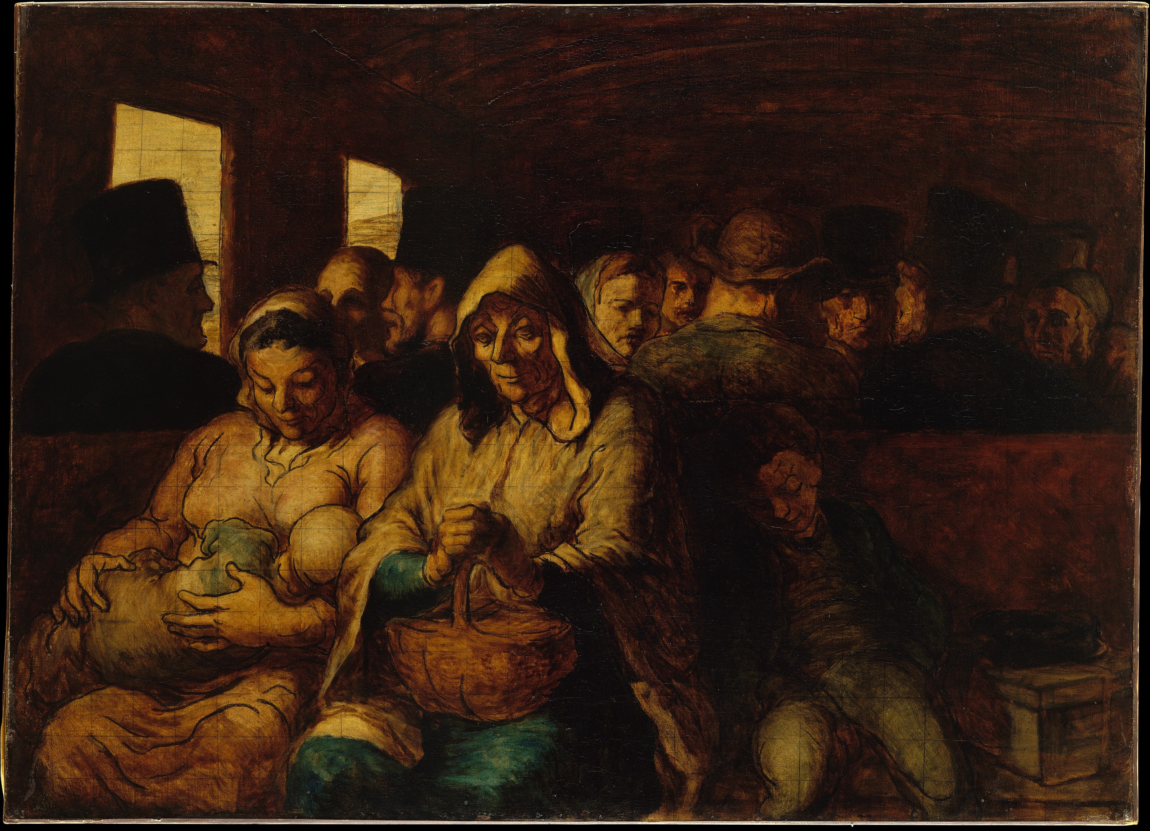
The Third-Class Carriage is a c. 1862–1864 oil on canvas painting by Honoré Daumier
Jules Dupuit’s 1849 comments of the railroad industry in France:
It is not because of the few thousand francs which have to be spent to put a roof over the third-class carriages or to upholster the third class seats that some company or other has open carriages with wooden benches. What the company is trying to do is to prevent the passengers who pay the second class fare from traveling third class; it hits the poor, not because it wants to hurt them, but to frighten the rich.
(Indirect source: ‘Quantum Microeconomics’)
There is typically lots of discussion of this in the media, see e.g., THIS article in The Economist
5.11.1 Formal characterisation (O-R)
The self-selection problem is characterized by a ‘menu’ of items that the firm offers, each item having a price and a quantity (or level of quality). To achieve the desired “self selection”, as implied above, several ‘constraints’ must be met. These constraints are necessary so that each of the consumers prefers to choose the item ‘intended for them’ (rather than another menu item), and also wants to buy something rather than nothing.
Following O-R, we present a somewhat general definition, and then prove and discuss results for a two-consumer case. (Time-permitting: parametric examples.)
This is an example of an asymmetric information problem: the consumer has more information about her own value then does the monopolist. This setup is also mathematically equivalent to a general class of “principal agent” and “hidden information” problems. If you further study ‘agency theory’, ‘contract theory’, or ‘mechanism design’, you will see this setup again. This is a workhorse setup in modern microeconomics. For a standard treatment of the ‘hidden information’ problem, see my slides HERE, with content drawn from Laffont and Martimort, 2002, and Salanie, 2005.
First a fairly general definition of ‘a monopolistic market with a menu’ from O-R, allowing for any number of consumers with distinct valuations of each of the different quantities of the good:
Demand
The function \(V_i\) is the value function for consumer \(i\), giving the maximum amount \(V_i (q)\) consumer \(i\) is willing to pay for \(q\) units of the good.
This is similar to value functions we’ve seen before.*
*Consider the ‘contribution to utility’ made by the consumption of a single good, holding other consumption constant, as expressed in the ‘units of other goods one would be willing to give up’.
Defining these value functions
A collection \((V^i)^n_{i=1}\) of increasing continuous [value] functions, where \(V_i : [0,1] \rightarrow R^+\) and \(V_i(0) = 0.\)
To consider this most simply, they ‘normalise’ the units of ‘quantity of the good’ (or ‘quality of the good’) to fall between 0 and 1, including the endpoints (that’s what the closed set \([0,1]\) denotes).
They normalise the value of consuming 0 units to 0, for all types of consumer.
Note that, as these are increasing functions, each consumer’s value is increasing in the amount consumed, up to a maximum value at 1 unit consumed.
I keep mentioning that this can also express units of quality (rather than quantity). The problem is mathematically equivalent if, as is commonly seen in the real world, a firm uses product quality to get consumers to self-select.
Producer
A single producer, called a monopolist, with no costs, who chooses a set \(M\) of pairs, called a menu, where a pair \((q,m)\) represents the option to buy q units of the good at the (total) price \(m\).
Each consumer chooses whether to buy one item on this menu, or nothing at all:
If \(V_i(q)−m ≥ 0\) for some \((q,m) \in M\), consumer \(i\) chooses an option \((q,m) \in M\) for which \(V_i(q)−m\) is maximal; otherwise she buys nothing.
The producer chooses M [the set of menu items] so that the consumers’ choices maximize her profit.
Problems like this are often stated in terms of the firm (or “principal”) choosing the values of the menu elements to maximize their payoffs subject to certain constraints. The problem is broken up into two parts –
- We consider each of the different ‘implementations’, i.e., the ways a firm might want get consumers to self-select into choosing different menu items.
For example…
Considering a set of consumers with ‘high’, ‘medium’, and ‘low’ valuations of each unit of the product, where there is no overlap in valuations:
‘Fully separating’… each of the three types of consumers may select a different menu item, perhaps the highest value select the highest cost and largest menu item, the medium select the medium item, and the lowest value consumer select the cheapest and smallest item.
‘Fully pooling’… all of the consumers select the same item
‘Partial pooling’… The high and medium value consumer select the same item, while the low value consumers select a smaller and cheaper item
‘Partial shut-down’ or the the high and medium value consumers may select different items, while the low value consumers do not purchase anything at all, they are ‘shut down’.
For a general class of cases it can be shown that the fully pooling outcome is not profit-maximizing.
- Given the chosen ‘implementation’, we consider the maximum profit the firm can make with this implementation. It cannot simply choose any price and any quantity for each menu item. To achieve a particular set of consumer choices (to pool, separate, etc), it will need to consider two constraints on the menu:
‘Incentive Compatibility (IC) constraint’: Among the items on the menu, each consumer must gets the greatest payoff from making the choice that the firm wants it to make (rather than by choosing another menu item).
‘Participation constraint’ (PC): Each consumer must prefer to choose the menu item the firm wants it to choose over “not participating at all”, i.e., over not buying anything.
The participation constraint is sometimes referred to as the individual rationality (IR) constraint.
To find the most profitable strategy, we need to consider all of the possible implementations, determine the profits from each, and find the implementation that yields the greatest profits.
The O-R example below is somewhat unusual. I intend to add a more standard parametric example here, with an algebraic as well as a graphical depiction, both in text and in a video.
Exeter video: Self-selection (2nd degree PD); informal graphical presentation
5.11.3 Two consumer self-selection: a simpler parametric example
This draws from Laffont and Martimort (2002), section 2.1.5.2, which in turn draws from Maskin and Riley (1984)
The firm
Suppose the firm produces at a marginal cost \(c\) per unit, and no fixed costs, thus its profit when it charges \(t\) for quantity \(q\) is
\[V(t,q) = t - cq\].
Consumers
(From Laffont and Martimort, notation adjusted:)
The tastes of a buyer for the private good are such that his utility function is \(U = \theta u(q) − t\), where \(q\) is the quantity consumed and \(t\) his payment to the principal. Suppose that the parameter \(\theta\) of each buyer is drawn independently from the same distribution on \(\theta = \theta_l, \theta_h\) with respective probabilities \(1-v\) and \(v\).
For ‘our example’, suppose \(u(q) = q^{1/2}\), \(\theta = \{1,2\}\) and \(v = 1/4\). Here we would have a \(1/4\) probability of a ‘high-type’ consumer who gets value \(2q^{1/2}\) from \(q\) units, and the remaining \(3/4\) probability of a ‘low-type’ consumer who gets value \(q^{1/2}\) from \(q\) units.
Let’s also define \(\Delta\theta = \theta_h- \theta_l\), the proportional difference in value of each unit for the high versus low type. For ‘our example’, \(\Delta\theta = 1\), implying that the high type always gets twice as much value from a particular quantity (or quality) as the low type.
Suppose that the firm offers two menu items:
In fact, as discussed elswehere, it is never optimal for the firm to offer more menu items than types of consumers, at least as long as the consumers are optimizing in a standard sense.
- \(q_l\) units of quality (or quantity) for price \(t_l\),
- \(q_h\) units of quality (or quantity) for price \(t_h\),
…and suppose the low-type consumer chooses the first menu item and the high-type consumer the second item.
We can now define the ‘rents’ (i.e., value of the good less the price paid) of the low (\(l\)) and high (\(h\)) type consumer as:
- \(U_l = \theta_l u(q_l) − t_l\) and
- \(U_h = \theta_h u(q_h) − t_h\),
respectively.
To induce these menu choices, both consumers must want to purchase their intended menu item. Each consumer most prefer this
- over ‘not buying anything’ … the ‘participation constraint’ (PC) and
- over ‘buying the other menu item’ … the ’incentive compatibility constraint (IC).
(Let the ‘rent’ from not buying anything equal to 0.)
Specifically, we need:
\[\begin{aligned}
U_l \geq 0 \:\:\:\:\:\:\:\: [PC_l]\\
U_h \geq 0 \:\:\:\:\:\:\:\: [PC_h]\\
U_l \geq U_h - \Delta \theta u(q_h) \:\:\:\:\:\:\:\: [IC_l]\\
U_h \geq U_l + \Delta \theta u(q_l) \:\:\:\:\:\:\:\: [IC_h]\\
\end{aligned}\]
Explaining the above:
\(PC_l\) and \(PC_h\): Recall our previous definition of the ‘rents’ (essentially willingness-to-pay in excess of price, i.e., ‘payoff’) for each type, \(U_l\) and \(U_h\). These must each be non-negative; each consumer must get at least as much value from their menu item as the price they pay for it.
\(IC_l\): The low-type’s payoff from chis own choice, \(U_l\), must exceed the payoff he would get from choosing the other menu item: \(\theta_l u(q_h) - t_h\). His payoff from this latter menu item equals the payoff the high type gets from this menu item *minus their differential value of this item \(\Delta \theta u(q_h)\), as he always values any quantity less than the chigh-type … thus \(U_l \geq U_h - \Delta \theta u(q_h)\) must hold.
\(IC_h\): The high-type’s payoff from her own choice, \(U_h\), must exceed the payoff she would get from choosing the other menu item: \(\theta_l u(q_l) - t_h\). Her payoff from this latter menu item equals the payoff the clow type gets from this menu item plus her differential value of this item \(\Delta \theta u(q_h)\), as she always values any quantity more than the low-type … thus \(U_h \geq U_l + \Delta \theta u(q_l)\) must hold.
As discussed in the previous section (and in more detail in the Supplement on Hidden Information), only \(PC_l\) and \(IC_h\) are binding (assuming we want to sell a positive amount to each type.) This implies they must hold with equality.
Thus \(U_l = 0\) and \(U_h = U_l + \Delta \theta u(q_l)\).
This tells us the ‘rent’ of the low type wil be 0, and the rent of the high type will be the difference in valuation of \(q_l\) between the types, which is positive if \(q_l\) is set to be positive.
Unpacking these, we have
\(\theta_l u(q_l) − t_l\) implying \(t_l=\theta_l u(q_l)\)
and we have
\(\theta_h u(q_h) = \theta_l u(q_l) − t_l + \Delta \theta u(q_l)\);
plugging in the \(t_l\) just derived (or noting \(U_l = 0\))…
\(\theta_h u(q_h) - t_h = \theta_l u(q_l) − \theta_l u(q_l + \Delta \theta u(q_l) = \Delta \theta u(q_l)\).
implying \(t_h = \theta_h u(q_h) - \Delta \theta u(q_l)\),
i.e. (unpacking the \(\Delta \theta\)) \(t_h = \theta_h u(q_h) - (\theta_h - \theta_l) u(q_l)\).
Note that as the quantity for the low type \(q_l\) is increased, \(u(q_l)\) increases (assume it’s an increasing function), and thus \((\theta_h - \theta_l)u(q_l)\), the ‘rent’ that must be left to the high type, to keep her from pretending to be the low type, must also increase. Thus \(q_l\) will not simply be set to trade off the value of the person who buys it against the marginal cost of production, but also in light of the incentive to avoid paying a rent … thus ‘distorted downwards’ in a wide set of cases.
Now we can consider the firm’s optimization problem:
\[\pi(t_l, t_h, q_l, q_h) = max_{t_l,t_h,q_l,q_h} (1-v) \times (t_l - cq_l) + v \times (t_h-cq_h) \] Subject to all of the constraints above.
Substituting in \(t_l\) and \(t_h\) implied by the binding constraints yields:
\[\pi(q_l, q_h) = max_{q_l,q_h} (1-v)(\theta_l u({q_l}) - cq_l) + v( \theta_h u(q_h) - (\theta_h - \theta_l) u(q_l)-cq_h)\] If this is a standard ‘concave problem’ (which will be implied by a concave value function \(u\)) we simply need to take the first-order-conditions wrt the choice variables \(q_l\) and \(q_h\).
Note \(q_h\) only enters into the part of the profit that comes from ‘when we actually are selling to a high type.’ Thus we simply find the (efficient) quantity where her marginal value equals the marginal cost:
\(v \theta_h u'(q_h) = vc \rightarrow \theta_h u'(q_h) = c\) … noting that \(\theta_h u'(q_h)\) represents the high-types marginal value at \(q_h\) units.
However \(q_l\) enters into the profit when we actually sell to a low type as well as when we sell to a high type. Taking the FOC (and re-using the ‘difference in value’ \(\Delta\) notation:
\((1-v)\times \big(\theta_l u'(q_l) - c\big) - v\times(\Delta \theta u'(q_l)\big)=0\)
Note that if only the first term were present, e.g., if \(v=0\) and we could price exclusively to the low type without worrying about the high type, we would choose the socially-efficient level of \(q_l\), trading off the marginal cost \(c\) against his marginal benefit, i.e., where \(\theta_l u'(q_l)=c\).
However, the second term causes the ‘downward quality’ (or quantity) distortion of \(q_l\) below this level. Rearranging this yields:
\((\theta_l-\frac{v}{1-v}\Delta\theta) u'(q_l)=c\), implying \(q_l\) must be less than the ‘first best’ \(q_l\).
Note that the greater the probability (\(v\)) of a high type, the greater the distortion of the low-type’s quantity.
It may be that even the first unit of \(q_l\) has too much of an effect on the information rent that must be paid to the high type to be worth offering. Here the above would solve to a ‘negative optimal \(q_l\), but the true optimal \(q_l=0\), the ’shut down’ policy.
Returning to ‘our example’, where \(u(q) = q^{1/2}\), \(\theta = \{1,2\}\) and \(v = 1/4\), implying \(\Delta\theta=1\), and letting \(c=1\):
\((1-\frac{1}{3}) \frac{1}{2} q_l^{-1/2} =\frac{1}{3} q_l^{-1/2} =1\)
\(\rightarrow q_l = 3^{-2} = 1/9\)
In contrast, if we could sell to the low-type in isolation (we knew his type … sort of ‘perfect price discrimination’) we would choose the efficient quantity according to:
\(\theta_l u'(q_{l,FB}) = c\), for our example implying the ‘First Best’
\(\frac{1}{2} q_{l,FB}^{-1/2} =1\)
\(\rightarrow q_{l,FB} = 1^{-2} = 1\).
Quite a distortion in this example!
5.12 How do firms actually price? (this section is a work in progress)
Some resources:
‘Pricing college’ podcast offers some insight into how firms and consultants tackle the issue of pricing, and some of the terminology that they use
Relevant but somewhat challenging:
References
Aguirre, Inaki, Simon Cowan, and John Vickers. 2010. “Monopoly Price Discrimination and Demand Curvature.” American Economic Review 100 (4): 1601–15.
Bergemann, Dirk, Benjamin Brooks, and Stephen Morris. 2015. “The Limits of Price Discrimination.” American Economic Review 105 (3): 921–57. https://doi.org/10.1257/aer.20130848.
Courty, Pascal, and Mario Pagliero. 2012. “The Impact of Price Discrimination on Revenue: Evidence from the Concert Industry.” Review of Economics and Statistics 94 (1): 359–69. https://doi.org/10.1162/REST_a_00179.
Cowan, Simon. 2012. “Third-Degree Price Discrimination and Consumer Surplus.” The Journal of Industrial Economics 60 (2): 333–45.
Kiser, E K. 1998. “Heterogeneity in Price Sensitivity and Retail Price Discrimination.” American Journal of Agricultural Economics. https://doi.org/10.2307/1244221.
Marsden, Ann, and Hugh Sibly. 2011. “An Integrated Approach to Teaching Price Discrimination.” International Review of Economics Education 10 (2): 75–90.
Varian, Hal R. 1985. “Price Discrimination and Social Welfare.” The American Economic Review, 870–75.
.svg)