8 Incomplete/Imperfect information (time permitting)

General progression through a game theory module or text:

As we consider progressively richer games, we progressively strengthen the equilibrium concept, in order to rule out implausible equilibria in the richer games that would survive if we applied equilibrium concepts suitable for simpler games (Gibbons, p. 173)

Nash Equilibrium (NE)\(\ \mathbf{\rightarrow }\) subgame-perfect NE (SPNE) $ Bayesian NE \(\mathbf{\rightarrow }\) Weak Sequential Equilibrium

Static games of perfect information \(\mathbf{\rightarrow }\) dynamic games of perfect (or ‘some imperfect’) information \(\mathbf{\rightarrow }\) static games of imperfect information \(\mathbf{\rightarrow }\)

dynamic games of imperfect information

We previously considered games were played was essentially simultaneous or entirely sequential. The important issue was whether or not a player knew the other players choice when making her choice (and potentially being able to revise for choice in light of this; see ‘subgame perfection’).

We assumed each player knew whom she would potentially be playing with, what her own payoffs were, and what the other players’ payoffs were.

We will now relax some of these assumptions to consider a wider class of interesting and relevant games. The notes below are less formal to allow us to get a taste of this material and the insights.

We will allow for:

1. (Asymmetric) “incomplete information” or (nature/chance); uncertainty about STATES: One or more players may not know for sure what the payoffs of other players are,* or (more or less equivalently) “who” the player she is facing is. However this is not blind “I do not know anything” uncertainty.**

* Or even she may be unaware of her own payoffs; There are even situations in which other players might know more about player’s payoff than the player herself (see for example models, in a slightly different context of “informed principals”).

** The latter is sometimes called ‘ambiguity’ or ‘Knightian uncertainty’.

Players know the probability of each type of payoffs, i., the distribution that the payoffs (or player types) are drawn from. This is often modeled in an extensive form or three form by having an initial player called “nature” who simply makes a random choice.

If we assume this is simple symmetric randomness, where all players are equally informed at all points in time, this can basically be encapsulated in our previous frameworks; simply replacing payoffs with expected payoffs.

Instead, we focus on cases where, at a certain point in time, one player knows more than the other player about the random realisation.

2. ‘Imperfect’ information about (some) previous moves (actions); uncertainty about ACTIONS

We have seen sequential games where players know all previous moves, i.e. they know “where in the game tree” they are when they make their choices. This was our standard extensive game. We have also seen that simultaneous games are equivalent to sequential games were no player is aware of the choices other players have made when they make their own choices.

Below, we will consider the case where some previous choices may be known while others are not.

We can depict “what a player knows when she made her choice” with the use of “information sets” also related to “information partitions”, described in the next subsection. In the tree diagrams these are usually depicted by connecting decision nodes (points where a player ‘has the move’) to one another with solid or dashed lines.

We may also consider ‘uncertainty about states’ with information partitions, if we use the aforementioned notation with the “nature” player.

8.1 Information sets (and ‘partitions’)

An information set for a player is a collection of decision nodes satisfying:*

*“An information partition is an allocation of each non-terminal node of the tree to an information set.”

1. The player has the move at every node in an information set

2. When the play of the game reaches a node in the information set, the player with the move does not know what node within the information set has (or has not) been reached

• The Player can not distinguish between nodes connected by an information set … because he/she doesn’t know what decisions were taken previously (by another player or by “nature”)

• A player can’t play a different strategy for different nodes connected by an information set

8.1.1 Examples in tree form

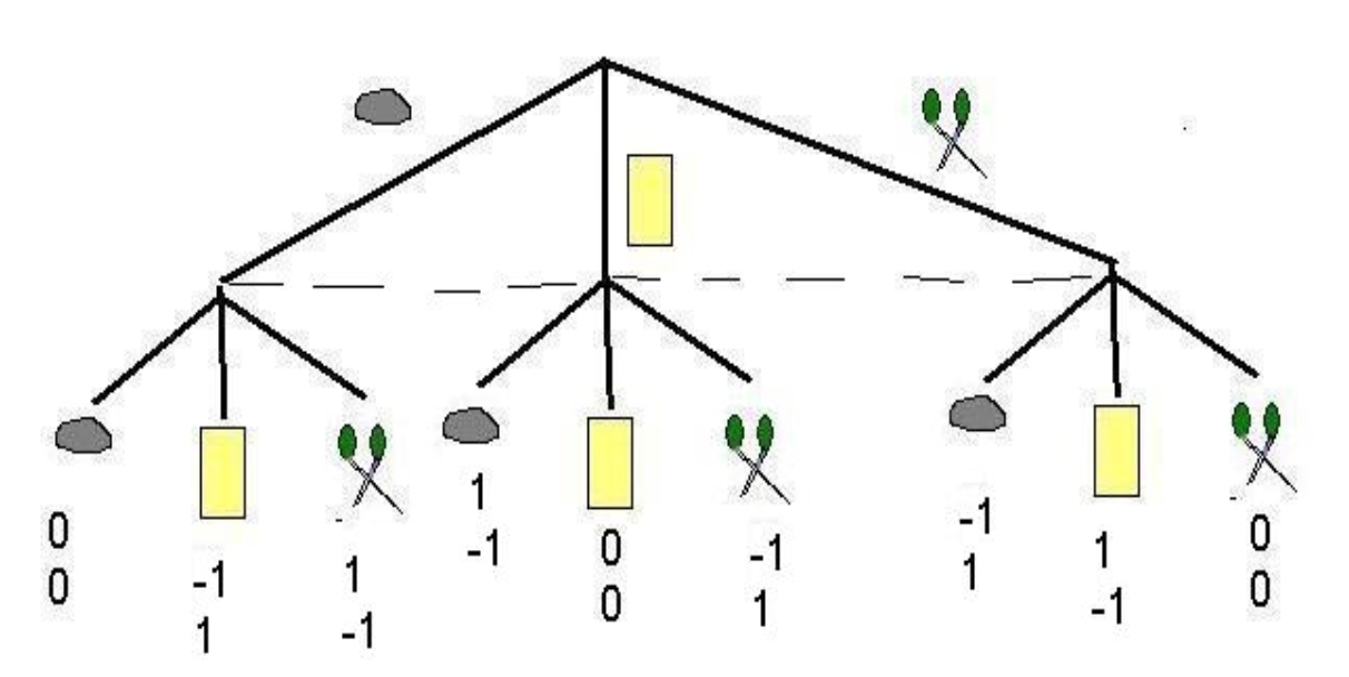
Example: ‘Rocks/Paper/Scissor’ in extensive form, with variations.

Traditional RPS:

Intuition: what are the NE?

This is a simultaneous ‘strictly competitive’ game.  This is an ‘anti-coordination’ game.

There can be no pure strategy NE.

If player 1 puts \(\frac{1}{3}\) probability on each player 2 is neutral between each action.. If player 2 puts \(\frac{1}{3}\) probability on each (of R, P, S) player 1 is neutral between each action.  Thus this is a NE, although there may other NE as well (I don’t think there are, but it is worth checking), using the techniques for simultaneous games we learned previously.

RPS where player 1 is very slow at making a fist:

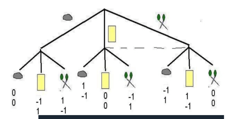
Intuition: What will occur?

If player 1 plays rock 2 will play paper and win, yielding payoffs of 0,1.

So player 1 probably won’t want to play rock.

But what will player 1 want to play? Paper or scissors?

If player 1 plays scissors or paper player 2 will not know which is played, and might play scissors (‘if not rock’), so as to either win or tie (but never lose).

But knowing this, player 1 might play scissors – but then 2 would want to play rock, which would mean 1 would want to play paper, which would mean 2 would want to play scissors, which would mean 1 would want to play scissors ... etc.

There would seem to be no pure strategy prediction here.

But there may be a mixed strategy NE in this ’subgame’.

8.2 Bayesian games (incomplete information, informal)

There is something uncertain, chosen by ‘nature or chance’ that affect the payoffs of one or more players (resulting from certain combinations of actions); typically we refer to this in terms of “types of players” where each type has a different set of payoffs that results from a certain profile of actions.

There are “common prior beliefs about types”: All players know the payoffs of each type and the probability of each type occurring. Furthermore, we typically assume all players know that all players know this, etc. (common knowledge).

However, one (or more) may know for certain which type she (or another player) is while other players may only know what the prior probabilities of this were.

E.g., perhaps we both know that there is a 25% chance that the player you will fight against will be strong (perhaps we can think of 1/4 of the ‘general population’). However, I know for certain whether I am strong or weak, while you do not know this, at the time you make your choice.**

** I am strong, by the way, not physically, but emotionally.

8.2.1 Bayesian Nash equilibrium (BNE; informal definition)

A BNE is a set of strategies, one for each type of player such that no type has an incentive to change his or her strategies given the beliefs about the types and what other types are doing.

See this ‘sourced’ video for a simple description, definition and numerical examples

E.g., fighting an opponent of unknown strength; Cournot competition between firms with unknown cost functions.

8.2.2 Example: Asymmetric information Cournot

This is a good example to start with but actually it is somewhat less interesting than other examples. This is because the payoffs for the ‘player with known costs’ actually don’t directly depend on the type of ‘unknown cost player’ player you are facing. They only depend on the strategy (here quantity) chosen by this player. So it simply becomes a sort of “average across the best responses to the quantity provided by each type you might be facing”.

A game like the yield-fight game (or equivalently, a simultaneous entry game) may be more interesting in this regard.

“Sourced” videos (unfold)

The video HERE presents a version of this game plugging in some specific numbers for certain parameters such as the probability of each type and the proportional cost for the low vs high type (1/2 in each case).

Sometimes playing your numbers make it easier to see the problem behind the notation and certainly easier to solve. However the limitation is that if you plug in specific numbers you can’t then look at “comparative statics” you cannot see how the results change as we adjust these parameters.

The video is correct but it is very slow (watch at 1.5 speed at least) and takes too many steps. He would be better off if he simply focused on the marginal revenue equals marginal cost condition and wouldn’t have to solve the problem for the low and high type separately.

Motivation:

Two firms choose quantities at the same time. One firm does not know whether the other firm is high or low cost, both know their own costs. Demand is linear, marginal costs are constant.

Q: How would you model this?

\[ \begin{aligned} P(Q) =a-Q=a-q_{1}-q_{2} \\ c_{1}(q_{1}) =cq_{1} \\ c_{2}(q_{2}) =c_{2}\cdot q_{2} \\ \text{Where} \text{: } \\ c_{2} =C_{H}\text{ with probability }\theta \\ c_{2} =C_{L}\text{ with probability }1-\theta \end{aligned} \]

Players: Firms 1 and 2*

* Alternatively, we can model this letting ‘Nature’ randomly choose 2’s type, if we want to use the extensive form/game tree).

Actions: Choose a quantity (\(q_{1}\) and \(q_{2}\))

Actions by types: \(1\) chooses \(q_{1}\)

Player \(2\), type \(c_{H}\) chooses \(q_{2}(c_{H})\)

Player \(2\), type \(c_{L}\) chooses \(q_{2}(c_{L})\)

Payoffs:

\[\pi _{k}=q_{k}\cdot p(Q)=q_{k}\cdot (a-q_{1}-q_{2}-c_{k})\text{ for }k\in \{1,2\}\]

States: Firm 2’s marginal cost \(c_{2}\in \{C_{H,}C_{L}\}\) where \(C_{L}<C_{H}\)

Information structure

\(2\) knows \(c_{2}\)

\(1\) has ‘beliefs’ that assign \(P(c_{2}=C_{H})=\theta\), \(P(c_{2}=C_{L})=1-\theta\)

Note: In these games, beliefs always correspond to the correct (correctly computed) probabilities given the information at hand.

Looking ahead…

In sequential games, as information is revealed, we will need to consider ‘correct Bayesian updating’, and we will look For “equilibrium assessments” combining strategies and beliefs at each node for each player…

where these beliefs at every point are consistent with the strategies chosen by each player (type of player) at each decision node.

Best Responses

Note: These will yield a NE strategy profile, a BNE outcome where these intersect,

Firm 2:

\(q_{2}^{\ast }(c_{t})\) solves \[\begin{aligned} \max_{q_{2}}\text{ }[(a-q_{1}^{\ast }-q_{2})-C_{t}]q_{2}\text{ for }t \in \{H,L\} \\ s.t.\text{ }q_{2} >0\end{aligned}\]

Q: Explain intuitively what firm 1 will do as a ‘best response’ ...

A: Firm 1 will set quantity to optimize its expected profit, knowing that there is some probability it will face a high-cost competitor, and some probability it will face a low cost competitor. The optimal quantity will be somewhere in between, in this case, in fact the weighted average of the optimal quantities in each case.

Firm 1:

\(q_{1}^{\ast }\) solves \[\begin{aligned} \max_{q_{1}}\text{ }\left\{ \begin{array}{c} \theta \lbrack a-q_{1}-q_{2}^{\ast }(C_{H})-c]q_{1}\text{ } \\ +(1-\theta )[a-q_{1}-q_{2}^{\ast }(C_{L})-c]q_{1}% \end{array}% \right\} \\ s.t.q_{1} >0\end{aligned}\]

Q: How to solve these for BR’s?

A: Solve for first order-conditions (set first derivative equal to zero).  This is a necessary condition for an interior optimum, though not sufficient. We want the ‘choice variable’ on the left hand side only, as a function of the parameters and the other firm’s choice.

FOC’s:

\[q_{2}^{\ast }(C_{t})=\frac{a-q_{1}^{\ast }-C_{t}}{2}\text{ for }t=L,H \tag{1 \ 2}\]

\[q_{1}^{\ast }=\frac{\theta \lbrack a-q_{2}^{\ast }(C_{H})-c]+(1-\theta )[a-q_{2}^{\ast }(C_{L})-c]}{2} \tag{3}\]

Note: This assumes the parameters are such that both quantities are positive.  Actually, we do have to worry about ‘corner solutions’ here – the high cost firm may not produce – but we ignore this for now.

Q: How to solve these for BNE quantities?

A: We need to solve this system of equations, substituting one player-type’s optimum into the others to find a ‘fixed point.’

Q: What will these BNE quantities be a function of?

A:They will be a function of the parameters (\(\theta ,c,C_{H},C_{L}\) ).  They will *not* be a function of the other player-type’s quantities!

We solve this by substituting equation 3 (\(q_{1}^{\ast }\)) into equations 1 & 2, and then substituting each of these (\(q_{2}^{\ast }(C_{L})\) and \(% q_{2}^{\ast }(C_{H})\)) into equation 3.  

This yields: \[\begin{aligned} q_{2}^{\ast }(C_{H}) =\frac{a-2C_{H}+C}{3}+\frac{1-\theta }{6}(C_{H}-C_{L}) \\ q_{2}^{\ast }(C_{L}) =\frac{a-2C_{L}+C}{3}-\frac{\theta }{6}(C_{H}-C_{L})\end{aligned}\]

Question: What is interesting about these BNE outcomes (outputs)?

• The output for the high-cost type is higher than the high-cost type’s output in the complete information case (i.e., in the case where player 1 knew 2’s cost). Remember, this complete informationoutput was \(q_{i}^{\ast }=\frac{a-2c_{i}+c_{j}}{3}\) where \(c_{i}\) was own and \(c_{j}\) was the other firm’s cost.

• Similarly, the output for the low-cost type is lower than the low-cost type’s output in the complete information case.

• For both types the BNE output involves not only the cost of the player’s type, but the cost of the player’s other type!  Note that this was not true for the BR functions!

Why?

A: Your optimal output depends not only on your own costs but on your expectation of the other player’s output, and thus on how the other player will react to what it thinks are your costs!  

Firm \(2\) will produce less when its costs are high than when they are low, ceterus paribus.  However, if firm 1 is not sure firm 2’s costs are high, firm \(1\) doesn’t know how much firm 2 will limit its output and thus 1 will not increase its output as much as it would if it knew firm 2’s costs were high.  Firm 2 knows this, and thus does not limit its output as much.  This second effect – the response to firm \(1\)’s lack of information, is described by the second additive terms in the above...

We see this insight even more dramatically in the fight/yield game depicted here. In this case, there can be an equilibrium where the ‘weak’ player chooses ‘fight’, even though it could never be an equilibrium for her to do so in a game with complete and perfect information.

Q: What did we forget to compute?

Firm 1’s BNE strategy (action): \[q_{1}^{\ast }=\frac{a-2c+\theta C_{H}+(1-\theta )C_{L}}{3}\]

Note, this is like a response based on ‘average’ \(c_{2}\), i.e., \(\theta C_{H}+(1-\theta )C_{L}\). This is a special case: equivalence does not always hold!

8.2.3 Example: ‘fight or yield’/simultaneous entry

In the above example only a single player’s payoffs (to particular combinations of actions) depended on the uncertainty (i.e., on the type of this same player, Firm 2). Thus we simply needed to

• figure out what ‘the best response of each type of Firm 2 was’

• figure out what Firm 1’s best response was to ‘the response of the average of Firm 2’s responses’

… and find an intersection.

However, we could let both players payoffs depend on this uncertainty, say, on "one player’s type’. This brings an additional (interesting) strategic concern.

Consider a game where both players A and B can choose ‘Fight’ (Enter) or ‘Yield’ (Don’t Enter). Player B may be of the Weak or Strong type. Only B knows her own type but both know the specific probability, say \(\alpha\), that A’s will be weak and some probability A’s are strong.*

This could be likened to a game where firms may enter a market and if both enter only the stronger firm will survive.

• Suppose that when both yield the payoffs are zero for both.

• When A fights and B yields (or vice versa) the fighter gets \(2\) and the yielder gets zero.

• When both fight then the ‘winner’ depends on whether B is strong.

  • If B is strong then she wins and gains \(1\), while A gets \(-1\)
  • If B is weak then she loses and gets \(-1\), while A gets \(1\)

(Note that I assumed that there is some value lost in the fighting.)

If my payoff to a particular action profile depends on your type, then if a particular action (say ‘Fight’) is more likely to come from your ‘strong type’ than your ‘weak type’, I need to take that into consideration in my response! And remember, this is still a simultaneous game.

In general we speak of similar concepts like the ‘acceptance curse’ in dating:

Chade (2006) explored a search and matching environment where participants observe noisy signals of their partners’ types. He notes an “acceptance curse” resembling the winner’s curse from auction theory: a partner’s acceptance decision reveals information about their type.

• (Gall and Reinstein 2020)

… implying that ‘the person who accepts your offer’ is an average of ‘a worse type’ than the average person. (Sorry, this sounds harsh).

If B only fights when she is strong and not when she is weak (i.e., if only strong B-types fight)

• ‘A playing against someone who fights means his playing against someone who is strong’ and

• ‘A playing against someone who does not fight means his playing against someone who is weak’.

So for A, playing fight means: - \(\alpha\) share of the time facing a strong opponent, who fights (and thus losing, getting -1), and - \(1-\alpha\) share of the time facing a weak opponent, who Yields (and thus gaining +2)

On the other hand if B ‘always fights’ (whether strong or weak), then for A, playing fight means:

• \(\alpha\) share of the time facing a strong opponent, who fights (and thus losing, getting -1 payoff),

• \(1-\alpha\) share of the time facing a weak opponent (and thus winning, getting +1 payoff)

An example of this game, with slightly different payoffs, deriving the equilibrium under two possible cases is given in these notes

8.3 Sequential Games with Imperfect information

Some notes here; some notation comes from a different Osborne text, as well as a text by Watson

Motivating Example - ‘Multi-stage-game’

Consider the ‘Multi-stage-game’ depicted in the tree below.*

* Remember, the dashed lines indicate that player 2, if she has the move, does not know whether 1 chose C or chose D.

Think it through … what might we expect will happen? Does it make sense to think that 1 will choose E?

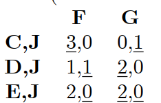
Or is a profile of strategies like \(\{C,J;F\}\) reasonable?

Intuition:

Action-wise, 1 can end the game early by choosing \(E\) and get a ‘safe’ payoff of 2. Or, she can choose D or C, which, as we see, can earn her a maximum payoff of 3, but a minimum payoff of 0.

If she chooses D or C, player 2 ‘has the move’ but 2 will not know whether D or C was chosen; 2 only will know that E was not chosen.

If 1 chose D then 2’s choice takes us to the terminal node; if 2 believes D was chosen she would prefer to choose F, leaving a payoff of only 1 to each player.

On the other hand, if 1 chose C, then if 2 chooses G the game ends and 1 gets 0 and 2 gets 1.

If, after C, 2 chooses F then 1 has the move once again. At this point 1 would prefer to choose J, earning 3 and leaving 0 for player 2.

So if 2 ‘gets the move’ we might think he will choose \(G\) if he thinks \(C\) was more likely chosen and she will choose \(F\) if he thinks \(D\) was more likely chosen. If 1 thinks that he can ‘fool’ 2 into thinking she chose D (and thus choosing F), she may want to choose C (and then J after F), to earn 3.

But should we predict that 2 is thus ‘fooled’? Would this be a reasonable ‘fool me once equilibrium’? We return to this below.

Above, suppose that player 1 plays the strategy highlighted in blue (player 2’s potential moves are in red). Given player 1’s strategy what should 2 suppose if he ‘gets the move’ (i.e., arrives at information set ${C,D}?

Let’s say (we are just considering this), that 2 supposes that “if 1 were to decide to deviate from his strategy (E,J) then 1 would play C with probability \(\frac{2}{3}\) and D with probability \(\frac{1}{3}\).”

• I.e., suppose 2’s beliefs at this information set assigned the probabilities \(\frac{2}{3}\) and \(\frac{1}{3}\) to C and D, respectively, as shown in brackets.

We assume that 2 will believe that, even after making this ‘mistake’ or ‘deviation’ 1 will subsequently play rationally, i.e., play J if she gets to the node following C,F. Indeed, the proposed strategy \((E,J)\) is consistent with this.

In fact, we will define the concept of sequential rationality to capture this; and n any strategy for player 1 that is ‘sequentially rational’ she must play \(J\) following the history \(\(C,F\)\),**

** We say ‘sequentially rational’ rather than ‘subgame perfect’ to also encompass decision nodes like the one faced by 2 when he has the move. Technically, these do not represent the initial node in a ‘subgame’ as the information set is not a ‘singleton’ … i.e., 2 doesn’t know ‘where he is’.

• and thus 2 must believe 1 will play \(J\) at this node in any WSE, for ‘Consistency of Beliefs with Strategies.’

*Given the assumptions above, and given 2’s beliefs (which we arbitrarily supposed) what is 2’s ‘best’ (sequentially rational) action at the information set \(\{C,D\}\)?

Let’s consider the Expected Utility payoffs to each move:

• If 1 played C, 2’s best move is G, yielding payoff 1. If 1 played D, G yields 0.

• If 1 played D, 2’s best move is F, yielding payoff 1. If 1 played C, F yields 0.

• \(\rightarrow\) So ‘which action is better’ depends on the probability 1 played C versus D

• We are supposing that (2 believes that), ‘off the equilibrium path’, C occurred with probability \(\frac{2}{3}\) and D with probability \(\frac{1}{3}\)

\(\rightarrow\) Thus 2’s EU payoffs to playing G are:

\[ \begin{aligned} EU_{2}(G) &=&\Pr (C)\times U_{2}(\{C;G\})+\Pr (D)\times U_{2}(\{D;G\}) \\ &=&\frac{2}{3}\times 1+\frac{1}{3}\times 0=\frac{2}{3} \end{aligned} \]

On the other hand, 2’s EU payoffs to playing F are:

\[ \begin{aligned} EU_{2}(F) &=&\Pr (C)\times U_{2}(\{C;F\})+\Pr (D)\times U_{2}(\{D;F\}) \\ &=&\frac{2}{3}\times 0+\frac{1}{3}\times 1=\frac{1}{3} \end{aligned} \]

So, given the assumptions above, given 2’s beliefs and 1’s optimal strategy (for the rest of the game), if 2 is at the information set ${C,D}$, his best move is \(G\). \(G\) is thus the ‘sequentially rational’ action given these beliefs and given 1’s strategy.

Hold on, you! If 1 is choosing \(E\) anyway, why do we need to worry about this?

Well, we are only considering that 1 may play E.

1 must ask ‘is playing E the best?’ ’Will playing C or D do better (in EU terms)?’

To get the answer to this question, 1 needs to ask ‘if I play C (or D), what will player 2 do?’

But what player 2 does at \(\{C,D\}\) will depend on what player 2 believes 1 played – \(C\) or \(D\).

So, in order to decide the EU payoffs to playing \(C\) (or \(D\)), to compare this to playing \(E\), 1 needs to know (or assign) what player 2’s beliefs are at \(\{C,D\}\).

Remember that ‘1 choosing (E,J)’ is a complete strategy, but this tells us nothing about what 2 is supposed to believe if he “gets the move”!

Motivating example: Sequential Rationality

I present this example to intuitively justify the reasonableness of the ‘Sequential Rationality’ requirement which will be part of the ‘Weak Sequential Equilibrium’.

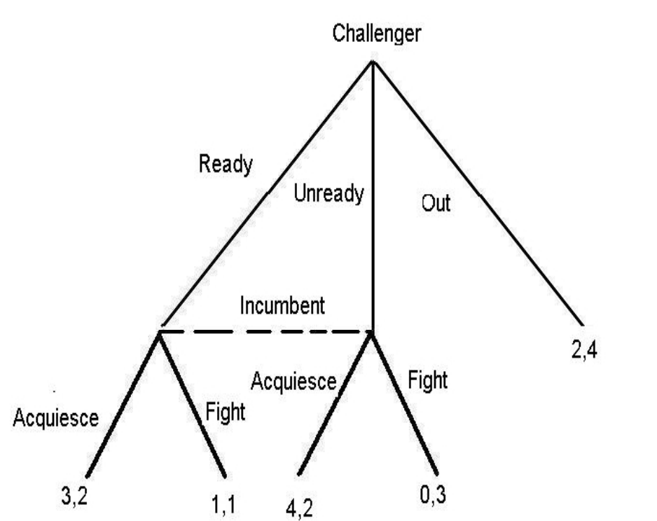
Consider the following example… Entry Readiness Game 1 with a Challenger who may be ready or unready and an Incumbent, depicted in the tree below.

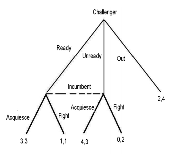
Entry Readiness Game 1

Note: Technically, there are no proper subgames (remember, a subgame must begin at a singleton information set). So SPNE is in fact the same as NE here.

Strategic form:

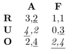
There are two NE here: \(\{Unready;Acquiesce\}\) and \(\{Out,Fight\}\).

Are they both reasonable?

Subgame perfection doesn’t eliminate either (no proper subgames).

But we know it is suboptimal for the incumbent to fight once the challenger has entered, whether or not the challenger is prepared. So ‘fight’ wouldn’t seem to be a good strategy ever, and thus ${Out; Fight}$ depends on an incredible threat.

We could add a requirement:

Optimal at each information set (Sequential Rationality): Each player’s strategy is optimal, given her beliefs, whenever she has the move.

I.e., each player’s strategy must be optimal at each of her information sets.

The strategy ‘Fight’ is not optimal at each information set here.

Why not?

A: it is not optimal for the incumbent to play Fight at the incumbent’s information set (when he has the move, i.e., after some form of entry). It is not if he is at the node following Unready nor if he is at the node following Ready. Thus, no matter his beliefs, this cannot be optimal.

Thus, only the NE strategy profile \(\{Unready; Acquiesce\}\) meets the (sequential rationality) requirement of optimality at each information set in the game above.

8.3.1 Definitions: Beliefs, sequential equilibrium, assessments

Remember: In simultaneous (static) games beliefs about other players’ strategies were ‘correct’ in equilibrium. No player ‘regretted’ her action.

For extensives game this idea is less clearly defined – some nodes are never reached, so there is no obvious ‘correct’ belief for nodes that are never reached in equilibrium !

\(\rightarrow\) We will define equilibrium in terms of pairs (assesments): Strategy profiles & collections of beliefs

Beliefs

At an information set with more than one history (element/node) the player who has the move ‘forms a belief over the histories’ (previous moves; including moves by nature).

At each information set a belief assigns a probability to each possible history,

or assigns a probability distribution over all the possible histories (in an infinite strategy set game)..

Belief System

A belief system is a collection of beliefs, one for each information set of each player.

Assessment

An assessment pairs a profile of strategies and a belief system.

Motivating example: Consistency of Beliefs

Consider the following variation of the previous entry game, depicted in the tree below. Call this ‘Entry Readiness Game 2’.

I present this example to intuitively justify the reasonableness of the ‘Consistency of beliefs’ requirement which will be part of the ‘Weak Sequential Equilibrium’.

Entry Readiness Game 2

Strategic form:

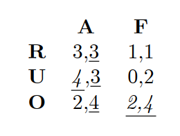
Now the incumbent prefers to fight if the challenger enters unready, but prefers to acquiesce if the challenger enters ready. So there is no clear optimal move at this information set – it depends whether or not the challenger prepared.

So, is \(\{Out; Fight\}\) a reasonable equilibrium profile?

Perhaps if the incumbent thinks ‘any challenger who enters will not prepare.’ At this node (following Unready) the action ‘Fight’ is optimal.

Thus the requirement of ‘optimality at each information set’ does not rule anything out here.

Note that whether fight is ‘optimal’ and thus whether the above can be an equilibrium profile depends on the incumbent’s beliefs about out-of-equilibrium play!

But are any beliefs reasonable? We have more to say on this…

8.3.2 Equilibrium Concept: Weak sequential equilibrium

WSE is ‘almost’ the same as Perfect Bayesian Equilibrium, which is more widely referred to. However, PBE imposes additional restrictions on out of equilibrium beliefs.

An assessment is a WSE if it meets two requirements

Requirement 1– Sequentially rationality: Each strategy is optimal for each player when he has the move given his belief (and the other players’ subsequent prescribed ‘continuation’ strategies)

Sequential rationality rules out off-the-equilibrium-path behavior that is ‘suboptimal’ (given ones beliefs and given the actions specified by the other players’ strategies)

Requirement 2 – Consistency of Beliefs with Strategies: Each player’s belief is consistent with the strategy profile See next section..

8.3.3 Consistency of Beliefs with Strategies (Requirement 2 of WSE)

In a steady state, each player’s belief must be correct’

• Osborne text

Consistency of beliefs at information sets:

At each information set beliefs are determined by Bayes’ rule and the players’ equilibrium strategies ‘where possible’.

Bayes Rule: *

* This is a fundamental rule of probability. It is very useful in a wide variety of contexts. It is worth digging into deeply and understanding it both formally and intuitively, and being able to apply it.

\[\Pr (X|Y_{1})=\frac{\Pr (X,Y_{1})}{\Pr (Y_{1})}\]

This can be thought of as the ‘definition of conditional probability’. But conditional probability also has an intuitive meaning.

We can also ‘invert the relationship’:

\[Pr(Y_{1}|X)=\frac{\Pr (X,Y_{1})}{\Pr (X)}=\frac{\Pr (X|Y_{1})\Pr (Y_{1})}{ \Pr (X)}\]

If \(Y\) is drawn from a discrete set of N possible events \(\mathbf{Y=}\{Y_{1},Y_{2},...,Y_{N}\}\) we have:

\[Pr(Y_{1}|X)=\frac{\Pr (X|Y_1)\Pr (Y_{1})}{\Pr (X|Y_{1})\Pr (Y_{1})+\Pr (X|Y_{2})\Pr(Y_{2})+...+\Pr (X|Y_{N})\Pr (Y_{N})}\]

For an interesting example, see the famous ‘false positives in a medical test’

Bayes rule for conditional probabilities in the present game theory case:

\[\Pr(h^{\ast}|I_{i}\text{ reached; strategy } \beta) =\frac{\Pr (h^{\ast };\beta )}{\sum\limits_{h\in I_{i}}\Pr (h;\beta )}\]

Read this as “the probability of a particular history \(h^{\ast}\) having occurred, given that a player finds herself at information set (node) \(I_{i}\), given all players’ strategies \(\beta\)”

Note \(Pr(h^{\ast },I_{i})=Pr(h^{\ast })\) here since these only occur together.

A player finds herself at information set \(I_{i}\). What probability should she assign that \(h^{\ast }\) has been played?

By the above formula, she should take the ratio of

• …the (unconditional) probability that \(h^{\ast }\) is played under the strategy \(\beta\)

• to the probability we get to the information set \(I_{i}\).

Note that the latter is the sum of the probabilities of each history that leads us to \(I_{i}\)… under strategy \(\beta\)).

Intuition: there may be multiple paths (histories( that could have lead to the information set \(I_i\). We are simply dividing the overall probability of history \(h^{\ast}\) (which leads \(I_i\)) by the sum of the probabilities of all other histories that lead to \(I_i\).*

This is only an interesting calculation if we have a mixed or “behavioral” strategy (similar to a mixed strategy but mixing at a particular information set/node). Otherwise the probability will generally be 1 or will be undefined.

Example: Consistency of beliefs at information sets “on the equilibrium path”

We come back to ‘Entry Readiness Game 1’:

Above, we decided that ${Unready,Acquiesce}$ and ${Out,Fight}$ are both SPNE, but only \(\{Unready,Acquiesce\}\) involves optimal actions at all information sets (‘continuation games’).

Let’s consider the (candidate) equilibrium ${Unready,Acquiesce}$, which is a SPNE, is optimal at each information set, and potentially also a WSE.

The incumbent’s information set ${Ready, Unready}$ is thus on the equilibrium path.

Given the challenger’s equilibrium strategy (if this is an equilibrium),

the only belief that is consistent with this strategy sets \(\Pr (Ready)=0,\Pr(Unready)=1\).

...And given this belief, the incumbent is playing the sequentially rational strategy ‘acquiesce.’

Example II : Consistency of beliefs at information sets “on the equilibrium path”

We return to the ‘Multi-stage-game’ depicted above:

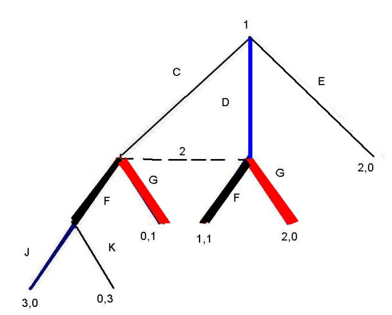
Multi-stage-game

1. Let’s examine the pairing of beliefs and strategies graphically depicted above.

• Player 1’s strategy (E,J) is depicted in blue.

• Player 2’s strategy is (G), depicted in red.

We already noted (see above discussion) that each of these strategies are sequentially rational (requirement 1).

Now…

Do player 2’s beliefs meet the consistency requirement (requirement II)?

Yes, they do trivially, because player 2’s information set is off the equilibrium path, so any beliefs are permitted.

So the assessment that pairs the profile of strategies \(\{E,J;G\}\) with player 2’s beliefs – \(\Pr (C)=\frac{2}{3}\),\(\Pr (D)=\frac{1}{3}\) is a WSE.

2. What about the profile \(\{D,J;G\}\) (depicted below)– This is a NE, and sequentially rational for the previously discussed belief system – \(\Pr(C)=\frac{2}{3}\),\(\Pr (D)=\frac{1}{3}\).

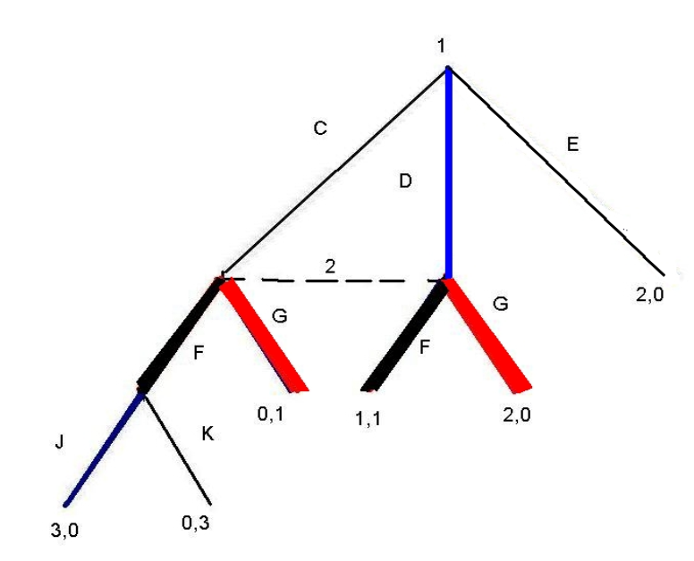
Multi-stage-game

But given 1’s strategy such a belief system is not consistent, as this ‘mixing’ does not describe what player 1 does, and this is on the equilibrium path!

Can this be a WSE for some consistent belief system?

Given 1’s strategy (D,J), the only consistent belief at information set \(\{C,D\}\) is simply \(\Pr (D)=1\).

But if \(\Pr (D)=1\),

\[\begin{aligned} EU_{2}(G) &=&0 \\ EU_{2}(F) &=&1 \end{aligned}\]

So playing G is not sequentially rational.

So the WSE rules out the ‘fool me once’ outcome we discussed at the top.

Note on the above, relating equilibrium concepts (unfold)

Remember: WSE is a refinement of SPNE, which was a refinement of NE. So, any PBE must be a SPNE and a NE (but not necessarily vice/versa)

Let’s examine a subset of the strategic form, leaving out strategies that include the strategy k (which cannot be part of a subgame perfect equilibrium).

Since \(\{E,J;G\}\) was the only SPNE in pure strategies we already knew it (paired with appropriate beliefs) was the only WSE in pure strategies.

8.3.4 Sequential games with ‘nature’

We now consider games where ‘chance plays a role’. As in our earlier discussion of ‘Bayesian games’, nature selects a random value which is revealed to (e.g.) only one player.

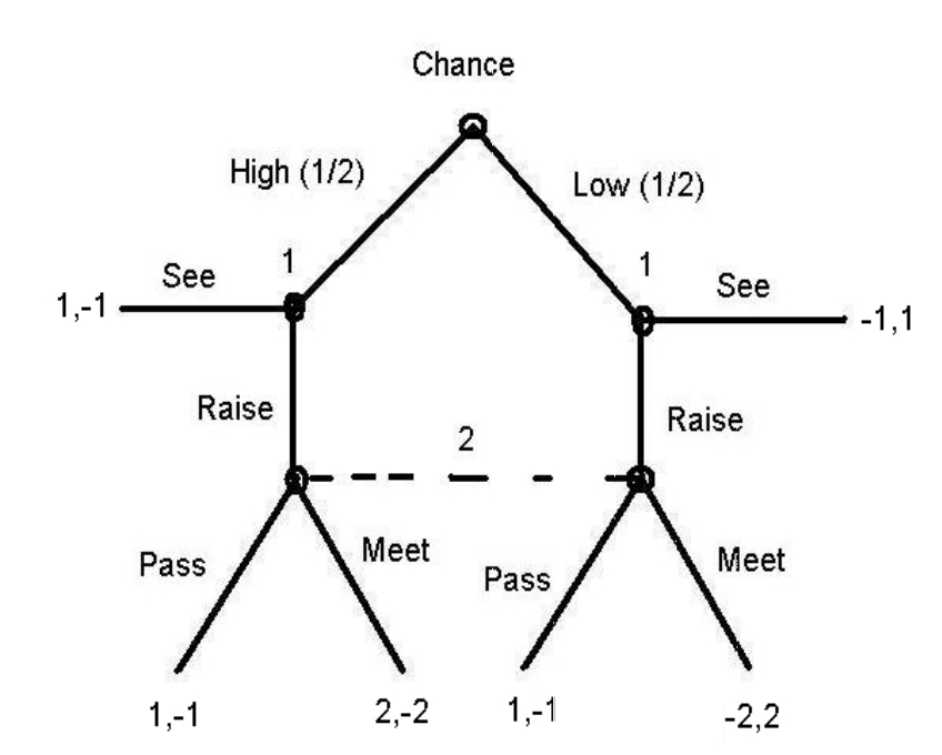
8.3.4.1 Example: (a very simplified version of) Poker

Nature first chooses whether player 1 has a ‘high’ or ‘low’ card (a good or bad hand) relative to the other player. She knows this.

She can ‘See’ (‘check’) or Raise the bet.

Next, player 2, who doesn’t know 1’s hand, can “Pass” (aka “fold his hand”) or “Meet”.

Payoffs are given below; note that these depend both on the actions of each player and on the ‘choice of Chance’.

We can write this in ‘Bayesian Normal (strategic) form’, to consider the BNE. Note that this does not consider sequential rationality:

Bayesian normal form:*

* Payoffs expressed as EU payoffs (over both types), player 1’s strategy depicted for ‘Low type, High type’ respectively

	Pass	Meet
R,R	1,-1	0,0
R,S	0,0	(1/2),-(1/2)
S,R	1,-1	-(1/2), (1/2)
S,S	0,0	0,0

\((S,S)\) is strictly dominated by a mixed strategy: \(\frac{1}{2} \cdot (R,R) \oplus \frac{1}{2} \cdot (R,S)\)

\(\mathbf{\Longrightarrow }(S,S)\) is not used as part of any NE

	Pass	Meet
R,R	1,-1	0,0
R,S	0,0	(1/2),-(1/2)
S,R	1,-1	-(1/2),(1/2)

\(\rightarrow\) No equilibrium in pure strategies.

\(\mathbf{\Longrightarrow }\Pr (meet)>0\)

\(\mathbf{\Longrightarrow }(S,R)\) not a BR:

–If Meet than (R,R) better

–If Pass than (R,R) is just as good

\(\mathbf{\Longrightarrow }\) So don’t put any probability on \((S,R)\); would do better by moving this to \((R,R)\)

\(\mathbf{\Longrightarrow }\) Mix between \((R,R)\) and \((R,S)\), which I claim was the intuitive result.

You will always raise if you have the high cards (there is no way to do better). You will sometimes raise if you have the low cards (i.e., ‘bluff’).

BNE strategy profile:

\((\frac{1}{3}\cdot (R,R) \oplus \frac{2}{3} \cdot (R,S); \: \frac{1}{3} \cdot p \oplus \frac{2}{3} \cdot m)\)

Player 1 bluffs with probability \(\frac{1}{3}\)… and player 2 ‘always calls bluff’ with probability \(\frac{2}{3}\).

Checking WSE for the above example

Is this a WSE (if paired with consistent beliefs?) Let us check our two requirements; we need only check these for player 2 given player 1’s strategy, since for player 1 we need not about beliefs or sequential rationality of his strategy.

1. Consistency of beliefs:

The only consistent beliefs at 2’s information set is that

(Recalling Bayes rule…:)

\(Pr(Y_{1}|X)=\frac{\Pr (X,Y_{1})}{\Pr (X)}=\frac{\Pr (X|Y_{1})\Pr (Y_{1})}{ \Pr (X)}=\frac{\Pr (X|Y)\Pr (Y_{1})}{\Pr (X|Y_{1})\Pr (Y_{1})+\Pr (X|Y_{2})\Pr (Y_{2})+...+\Pr (X|Y_{N})\Pr (Y_{N})}\)

Applying this to the present case:

\(Pr(\text{high} |\text{2 has move}) =\)

\(\frac{pr(raise|high)\ast pr(high)}{ pr(raise|high)\ast pr(high)+pr(raise|low)\ast pr(low)}=\frac{1\ast \frac{1}{2}}{1\ast \frac{1}{2}+\frac{1}{2}\ast \frac{1}{3}}=\frac{3}{4}\)

2. Sequential rationality:

If 2 plays Pass he gets \(-1\) (for sure)

If 2 plays Meet he gets \(-2\ast \frac{3}{4}+2\ast \frac{1}{4}= -1\)

So 2 is indeed neutral between these 2 strategies and thus mixing (in the proportions determined before) is a best response at this information set.

Hence, \((\frac{1}{3}\cdot (R,R) \oplus \frac{2}{3} \cdot (R,S); \: \frac{1}{3} \cdot p \oplus \frac{2}{3} \cdot m)\) paired with beliefs \(Pr(\text{high} |\text{2 has move}) =\frac{3}{4}\) is a WSE.

8.3.5 Most famous case: the (Spence 1973) signaling model

Simple 2x2 signaling game (education and labor market)

Players: Sender, Reciever, Nature

Actions (and order):

1. Nature: Good ability, Bad ability (chosen with probabilities \(P_{G}\) & \(1-P_{G}\))

2. Sender: Signal Good (e.g, School), Signal Bad (e.g., Drink)

3. Reciever: Hire, Not hire

Information structure:

Sender observes ability

Reciever does not observe ability (Nature’s move).

Receiver observes Sender’s signal.

Payoffs

In general

\(U_{\text{Sender}}= \text{Salary} - \text{cost of signal (a function of sender's ability)}\)

\(U_{Reciever}\)=

• If hire: Production (function of sender’s ability) - Salary

• If not hire: 0

In general, the production function and wages are such that the reciever will want to hire a good worker and not hire a bad worker.

However, if the receiver doesn’t know a sender’s (worker’s) ability, it would be more profitable to never hire than to always hire.

The overall structure is given below:

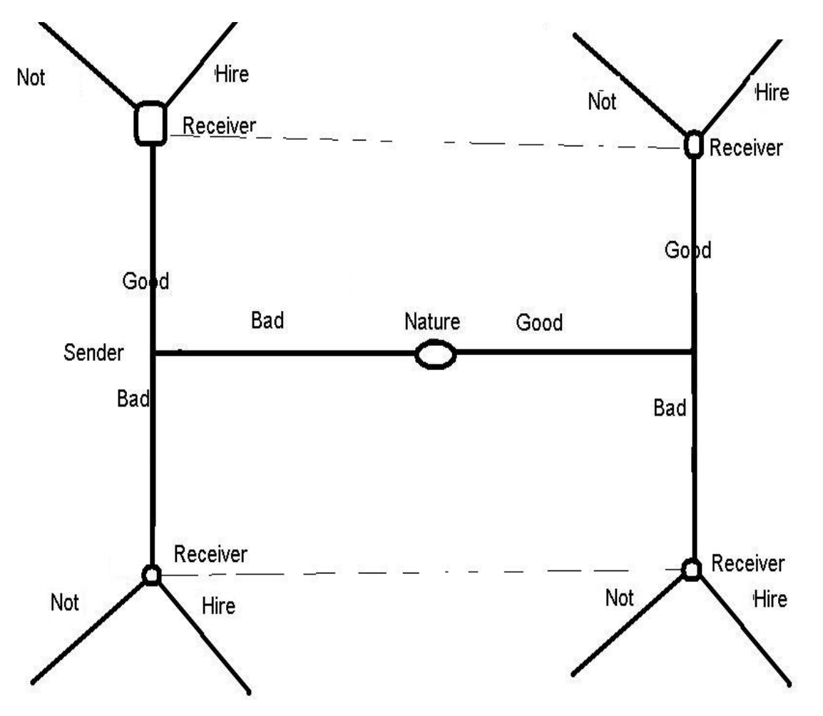
Figure 8.1: Signaling game structure

For a deep understanding of the signaling game we would want to analyze this game for all possible reasonable combinations of payoffs, and make some general conclusions that depend on the relative parameters.

For now, we will consider and contrast two numerical examples.

Signaling: Numerical Example I

Suppose the salary is set (exogenously) at \(S=4\).

The payoff to of not being hired is \(2\) (second best job).

The production of a bad worker is \(3\), so the firm ‘nets’ -1 from hiring such a worker.

The productivity of a good worker is \(6\), so the firm ‘nets’ 2 from hiring such a worker.

The cost of sending a good signal (e.g., going to school or university) is 1 for the good worker and 3 for the bad worker.

Finally, the probability of nature selecting a good worker is 0.1, i.e., 10%.

This implies the firm would rather hire a good worker but not hire a bad worker. However, the firm would rather hire no one than hiring everyone.

If education means the difference between a job or no job, in this case, only the good worker would choose to go to school (send a ‘good’ signal).

However if education will not make a difference (say, you are hired in either case), then neither type would go to school, as it is costly.

This yields the following game tree:

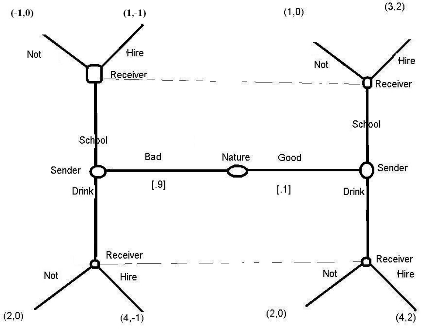
Figure 8.2: Signaling game example 1

Do you understand this setup? Can you describe the paths that lead to each terminal node?

Let us check a potential ‘separating’ equilibrium.

Suppose the Sender plays (Drink,School) – i.e., Drink if Bad, get an education if Good.

Then suppose the reciever plays (Not, Hire) – i.e., don’t hire if Drink, hire if School.

The only beliefs by a sender in such a situation that are consistent with this strategy is to believe Nature picked ‘Good’ if he receives a Good signal (School), and Nature picked ‘Bad’ if he receives a Bad signal (Drink).

Given these beliefs and strategies, are these best responses at each information set?

Compare Expected utility values:

\[EU_{S}(Drink,School;(Not,Hire))=0.1(4)+0.9(2)=0.2\]

Note this EU is additive in the EU of each ‘type’ (good or bad). Thus for this to be a BR it has to be a BR for each type of sender. We also require sequential rationality, which implies a player is acting optimally given his beliefs at each information set.

Note that given the receiver’s strategy (hire if and only if the sender is educated) the decision to get an education is pivotal. And as we set it up, only the good type wants to get an education if it is pivotal. So yes, each type of sender is behaving optimally (i.e., the sender is behaving optimally in each contingency)

Given the sender’s strategy (get education if and only if Good), is the reciever behaving optimally given her beliefs? Of course she is:

As we set it up, the receiver prefers to hire the Good, and not hire the Bad.

So this \(\{Drink,School;Not,Hire\}\) is a WSE (sequential rational under the beliefs mentioned above, which are of course consistent).

But this might not be the only WSE for this numerical example – there may be others. For example, pooling on ‘no school’ – if the employer will not hire for either signal – is a WSE. I.e., \(\{Drink,Drink; \: Not,Not\}\) paired with the belief \(\big(Pr(Good|Drink)=Pr(Good|School)=0.1\big)\) is a WSE.*

* Exercise: Check this.

Signaling: Numerical Example II

Let’s change the payoff:

Suppose the salary is set (exogenously) at \(S=5\)

The payoff to of not being hired is \(0\).

The production of a bad worker is 4, so the firm ‘nets’ -1 from hiring such a worker.

The productivity of a good worker is 7, so the firm ‘nets’ 2 from hiring such a worker.

The cost of sending a good signal (e.g., going to school) is 1 for the good worker and 2 for the bad worker.

Finally, the probability of nature selecting a good worker is 0.1.  

This implies (as before) the firm would rather hire a good worker but not hire a bad worker.

However, (as before) the firm would rather hire no one than hiring everyone; so if there is pooling, it must be involve hiring no one.

Notice: (Unlike before ) If education means the difference between a job or no job (i.e., is ‘pivotal’), both types would choose to go to school (send a ‘good’ signal).

However (as before) if education will not make a difference (say, you are hired in either case), then neither type would go to school, as it is costly.

This yields the following game tree: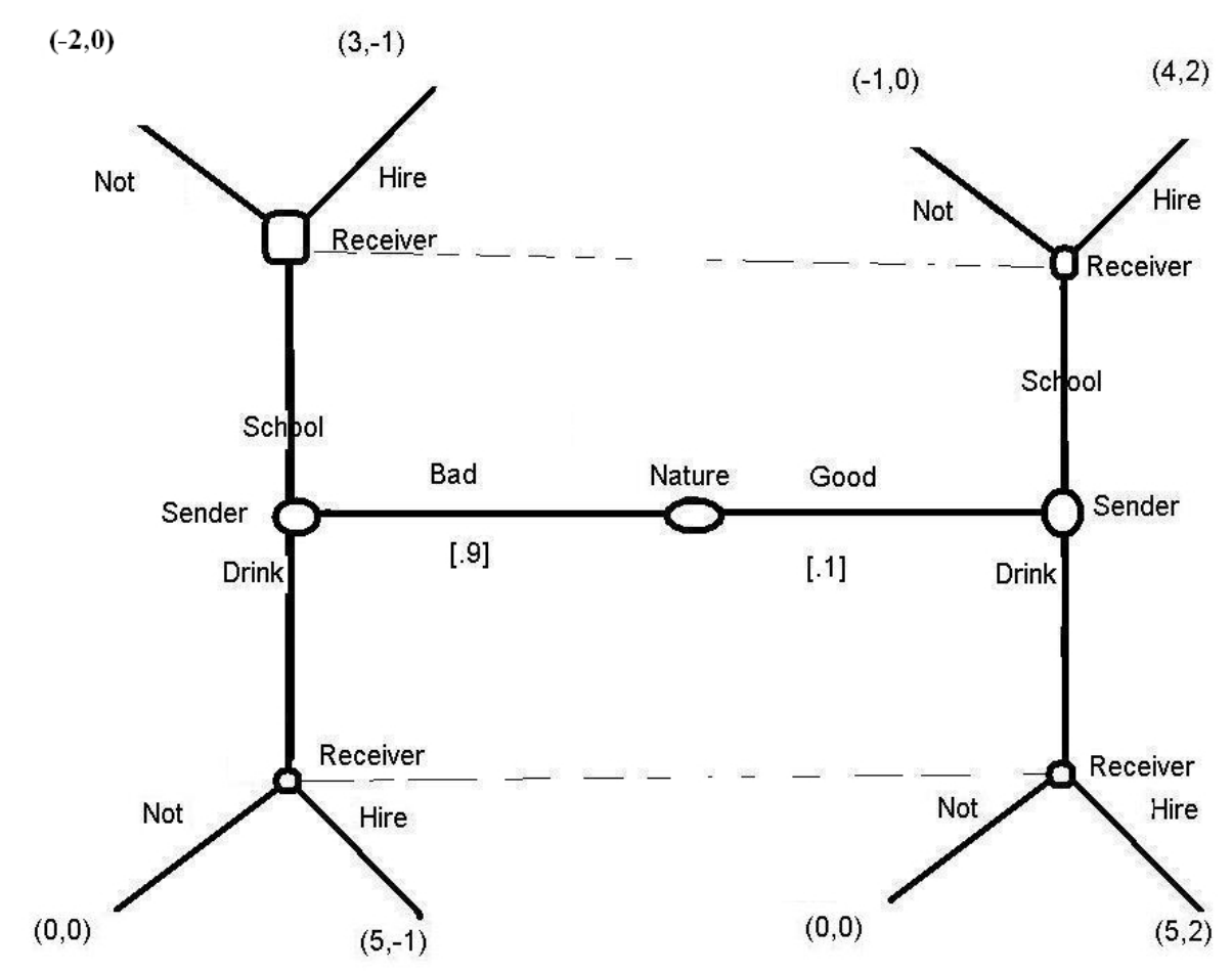

Figure 8.3: Signaling game example 2

Let us check a potential ‘separating’ equilibrium.

Suppose the sender plays (Drink,School) – i.e., don’t get an education if bad, get an education if good. Then suppose the Reciever plays (Not, Hire) – i.e., don’t hire if Drink, hire if School.

The only beliefs by a Reciever in such a situation that are consistent with this strategy is to believe Nature picked ‘Good’ if he receives a Good signal (education), and Nature picked ‘Bad’ if he receives a Bad signal (Drink).

Given these beliefs and strategies, are these best responses at each information set?

Note that given the receiver’s strategy (hire if and only if educated) the decision to get an education is pivotal. And, as we set it up, each type of sender wants to get an education if it is pivotal. So the sender is not behaving optimally in the contingency where he is Bad (i.e., for this type). The bad type should also want to pretend to be a good type and get an education. So this is NOT a WSE!

We can look for pooling WSE in this case – there seem to be no separating WSE (in pure strategies) here.

Note that the firm prefers to hire no one than hire everyone (given the setup). So, if both types do the same thing, the firm cannot tell which is which, and will thus hire no one. So for any pooling equilibrium here, the firm will hire no one. For example, we can look at {\(Drink,Drink; \: Not,Not\) }.

However, here the firm could assign any beliefs if it observes a good signal (education), as such a signal is off the equilibrium path.It gets complicated now.

One possible belief that the firm might hold is that any player who signals Good (gets an education) is a Good worker. But if this were the beliefs, the firm would not be behaving optimally – it should thus hire such a worker!

Another possible belief is that if a worker signals ‘Good’ it has only a \(.1\) probability of being a Good worker. I.e., the conditional probability (after observing such off-path play) is the same as the unconditional probability.This belief will make the strategy profile {\(Drink,Drink; \: Not,Not\)} sequentially rational. Thus {\(Drink,Drink; \: Not,Not\) } paired with the belief (\(Pr(Good|Drink) = Pr(Good|School)=0.1\)) is a WSE.

We can also look for other possible WSE. We may find a separating (or pooling) WSE where the receiver plays behavioral strategies, hiring only some proportion of the time when she gets a good signal. In such a case, the EU benefit to the sender may be such that getting an education is only pivotal for the Good type. This is too complicated to cover now.

Note: further study of signaling games and sequential games with asymmetric information would involve:

• Restricting the set of beliefs that are reasonable off the equilibrium path; this relates to the ‘Perfect Bayesian Equilibrium’ concept and to the so-called ‘Intuitive Criterion’

• Considering a “designer’s” choice of a cost of a signaling mechanism; How much should it cost and how can it fruitfully separate types without wasting too many resources?

• Considering equilibria involving ‘behavioral strategies’ as mentioned above.

References

Gall, Thomas, and David Reinstein. 2020. “Losing Face.” Oxford Economic Papers 72 (1): 164–90.

Spence, M. 1973. “Job Market Signaling.” Quarterly Journal of Economics 87 (3): 355–74. https://doi.org/10.2307/1882010.