4 Analysis focusing on ‘impact of impact information’
4.1 Code and data setup3
Links to experiment source, description, data characterization (ICRC Donor’s voice experiments: all input and description)
See ICRC donation suggestion and cost-info trial: Project description, summary, timing, background, other files linked within
Discussion of input, clean, mutate
The ‘input and cleaning’ (currently from stata dta) is now done in icrc_input_clean.R, which is run in main_all.R
Unfold details of data files, import to R, cleaning
Our charity partner (ICRC) gave us the file: List to be sent to deborah (2).xls (and a few others I don’t think we’re using).
Work done in Stata:
stata_do_files_linked/0_cleaning.do: Input from Excel file(s?) provided by ICRC. Cleaning, labelling, and scaling variables…
Note this also merges with earlier data on the giving behavior of these participants (input and cleaned elsewhere … todo: recover that code)
That work outputs data_grid_experiment_clean.dta, which is (Check: how was it moved here? Should we use a sourcing command for that?)
Import to R:
icrc <- readstata13::read.dta13 … convert dates, various factor options
source(here("dr_r_build_analysis_icrc_expt", "icrc_input_clean.R"))
… reads in data_grid_experiment_clean.dta, does some data cleaning, saves as data_icrc/edited_data/icrc.RDS
icrc <- readRDS(here::here("data_icrc", "edited_data", "icrc"))Set (and also get) names of key variables and objects to model
treatments_all <- levels(icrc$treatment)
treatments_impact <- c("Cost", "Cost_Sug_50", "Cost_Sug_150")
treatments_sug <- c("Cost", "Cost_Sug_50", "Cost_Sug_150")

outcomes <- c("d_don", "don_amt")

bin_outcomes  <- c("d_don")
cont_outcomes <- c("don_amt")

# TODO -- set of 'columns coded for meta-analysis' ... same across studies, if possible
Description/depiction/codebook of (summary) data
Key descriptives
Treatments: ControlCostCost_Sug_50Cost_Sug_150Sug_50Sug_150ICRC_Standard
Crosstab of treatment dimensions
icrc %>%
  tabyl(d_impact, sug_amt) %>%
tabylstuff()| d_impact | None | 50 | 150 | 50, 100, 150 | Total |
|---|---|---|---|---|---|
| 0 | 25.0% (24222) | 25.0% (24220) | 25.0% (24222) | 25.0% (24255) | 100.0% (96919) |
| 1 | 33.3% (24234) | 33.3% (24227) | 33.3% (24248) | 0.0% (0) | 100.0% (72709) |
| Total | 28.6% (48456) | 28.6% (48447) | 28.6% (48470) | 14.3% (24255) | 100.0% (169628) |
Donation incidence by treatment:
(
  don_shares <- icrc %>%
    tabyl(treatment, d_don) %>%
    tabylstuff()
)| treatment | 0 | 1 | Total |
|---|---|---|---|
| Control | 94.6% (22915) | 5.4% (1307) | 100.0% (24222) |
| Cost | 94.7% (22959) | 5.3% (1275) | 100.0% (24234) |
| Cost_Sug_50 | 94.5% (22892) | 5.5% (1335) | 100.0% (24227) |
| Cost_Sug_150 | 95.1% (23052) | 4.9% (1196) | 100.0% (24248) |
| Sug_50 | 94.6% (22921) | 5.4% (1299) | 100.0% (24220) |
| Sug_150 | 95.0% (23015) | 5.0% (1207) | 100.0% (24222) |
| ICRC_Standard | 94.9% (23024) | 5.1% (1231) | 100.0% (24255) |
| Total | 94.8% (160778) | 5.2% (8850) | 100.0% (169628) |
icrc %>%
  group_by(d_impact, sug_amt) %>%
  summarise(n =n(), `Pct. donating` = op(mean(d_don)*100, d=3))
## # A tibble: 7 × 4
## # Groups: d_impact [2]
## d_impact sug_amt n
## <fct> <fct> <int>
## 1 0 None 24222
## 2 0 50 24220
## 3 0 150 24222
## 4 0 50, 100, 150 24255
## 5 1 None 24234
## 6 1 50 24227
## 7 1 150 24248
## # … with 1 more variable:
## # `Pct. donating` <chr>The rate of making ‘some donation’ is 5.22% overall, and, as shown in the table above, this rate is similar across treatments.
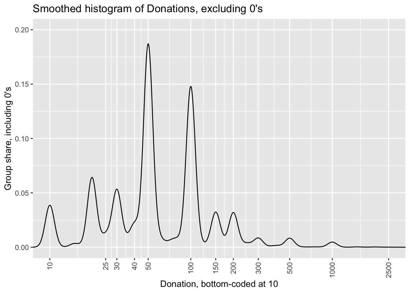
Below, we plot smoothed density plots of donations overall, focusing on positive donations. The graphs below do not show the zero-donation responses, which, as noted above constitute the vast majority of the population. However, the rates presented are as a share of all households, including non-donors.4
Next, we break this up by whether a ‘cost per impact’ measure was presented, pooling across suggested donation categories. Again, while the graphs do not show non-donors, the rates presented are as a share of all households in each grouping, including non-donors.
(
icrc_hist_treat_impact <- icrc %>%
    ggplot() +
     geom_density(aes(x=don_amt_bc10, y = after_stat(density), colour=d_impact)) +
        scales_theme +
   don_hist_label
)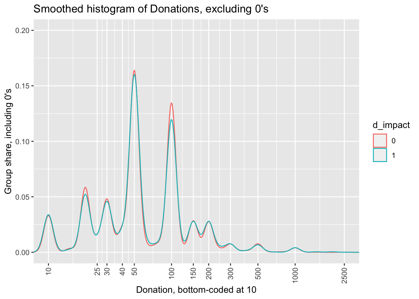
There is little visually-apparent difference in the donation patterns by the presentation of this information. We return to this more formally later.
(
icrc_hist_treat_sug <- icrc %>%
    ggplot() +
     geom_density(aes(x=don_amt_bc10, y = after_stat(density), colour=sug_amt)) +
        scales_theme +
   don_hist_label
)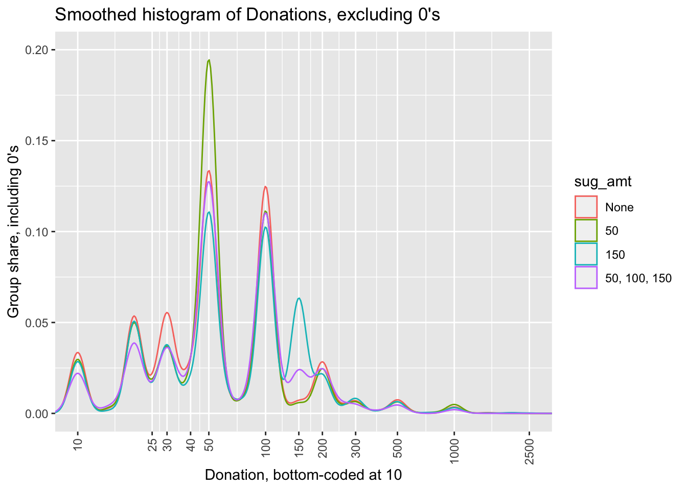
Here, we see some apparently stronger patterns. Unsurprisingly those offered a suggested donation of 50 seem, relatively and absolutely, more likely to donate 50, and similarly for those suggested 150.
This bears a closer inspection and formal analysis. We will do this elsewhere, as it is not the focus of the current project (although it was one of the two pre-registered focuses of this particular experiment.)
odd_dons <- sum(icrc$don_amt %nin% names(sort(table(icrc$don_amt), decreasing=TRUE)[1:11]), na.rm=TRUE)

tot_dons <-  sum(icrc$d_don)
Note that most donations are ‘round numbers’. As percentages of the 169628 households, the 11 most frequent donation amounts are:
94.78 1.51 1.20 0.52 0.42 0.26 0.26 0.25 0.16 0.08 0.07.
All other donation amounts account for only 818 donations, only 9.24% of all donations.
4.2 ICRC ‘impact information’ treatments: Questions and tests
Rather than poetically characterizing our results, we try to keep the narrative short to let the data and statistical measures speak for themselves. The tests below follow from the questions asked and procedures proposed in our pregistration.
In the preregistration we say …
We supplement this with exploratory work and robustness considerations.
This is followed by Bayesian inference probing the ‘tight bounds’ of the null effect.
This naturally connects to the (arguably, most important) section, conducting meta-analysis across related experiments.5
4.3 Preregistered tests
Note: these have (mainly/entirely) been done in 1_analysis_pap.do in the Dropbox folder Dropbox/ICRC_Fundraising/ICRC Grids Output Experiment/build_and_analysis/analysis/1_analysis_pap.do.
We may re-do some of these here for completeness.
4.5 Bayesian intervals, equivalence tests, probing the ‘tight null effect’
As our (above/linked) pre-registered analysis suggests, the effect of the cost impact information on incidence or amounts (CHECK) donated appears small, and it is far from statistically significant in conventional tests.
For this to be meaningfully informative, there are at least three key issues…
Manipulation check and external generalizability: Make a convincing case that these “cost impact” treatments were meaningful and represented ‘important, substantial, and relevant manipulations’. If these treatments were ‘as powerful, and of the sort that charities have used and could be expected to use in future’, a ‘null result’ could be useful.
Non-obviousness: Practitioners and social scientist’s prior beliefs (before our study) should have put some reasonably large probability that cost impact treatments would have a non-small effect in one direction or the other.
Tight statistical bounds: Any ‘underpowered’ study can ‘fail to reject the null’, and might also (even by chance) have a point estimate very close to zero. This does not make it informative.6 We need to demonstrate that, given our data and design ‘results as small as ours’ are very unlikely to have been generated, had their been an effect greater than some minimum size. Relatedly, we can use a Bayesian framework to demonstrate that ’with a range of reasonable prior beliefs over the true effect, one’s posterior belief after seeing our data, should put very low probability on an effect greater than some minimum size.
(We present the latter approach below, but I intend to also do a more frequentist Equivalence Test this with a simple randomization inference exercise.)
Bayesian Test of Difference in Proportions
Calibrating an ‘informative but centered prior’ over (independent) donation probabilities
In addition to a ‘flat (uniform) prior’ we consider a Beta prior that is centered roughly at the observed rate of donating, but allows what seems like a reasonable amount of dispersion.*
* We consider only priors that use the same distribution for the treatment and control groups, and (at least for now) assumes these are independent. Thus, our prior is not ‘baking in a likely effect in either direction’.
We give some calculations to get reasonable parameters for the beta distribution over the priors. We use the prevalence package, considering what seems a reasonable best-guess equal to the observed mean incidence, and 80 percent confidence it is between 1/3 of this and 3 times this.
p_load(prevalence)

mu_i <- mean(icrc$d_don)

beta_params_expert_i <- betaExpert(mu_i, mu_i/3, mu_i*3, p = 0.80, method = "mode")

a_e_i <- beta_params_expert_i$alpha
b_e_i <- beta_params_expert_i$beta
This generates an alpha of about 2.31 and a beta of about 24.9. This distribution has a mode exactly matching the empirical incidence rate of 5.22%, and a mean and median just a few percentage points above it. The standard deviation is nearly the same as the mode. We plot this density below.
beta_example_inf  <- data.frame(rbeta(10000, a_e_i, b_e_i)) %>% setnames("inf")
beta_example_inf_d <- density(beta_example_inf$inf) ##CHECK -- this seems to have negative values?


ggplot(beta_example_inf, aes(x = inf)) +  geom_density(n=10000)  +
  xlab("Value") +
  ylab("Density") +
  labs(title = "Beta Density (Informative for ICRC)") +
  theme(
    plot.title = element_text(hjust = 0.5),
    axis.text.y = element_blank(),
    axis.ticks.y = element_blank()
  ) +
  geom_vline(xintercept = beta_example_inf_d$x[beta_example_inf_d$y == max(beta_example_inf_d$y)],
             col = "red",
             size = 0.2) +
  coord_cartesian(xlim = c(0, .35))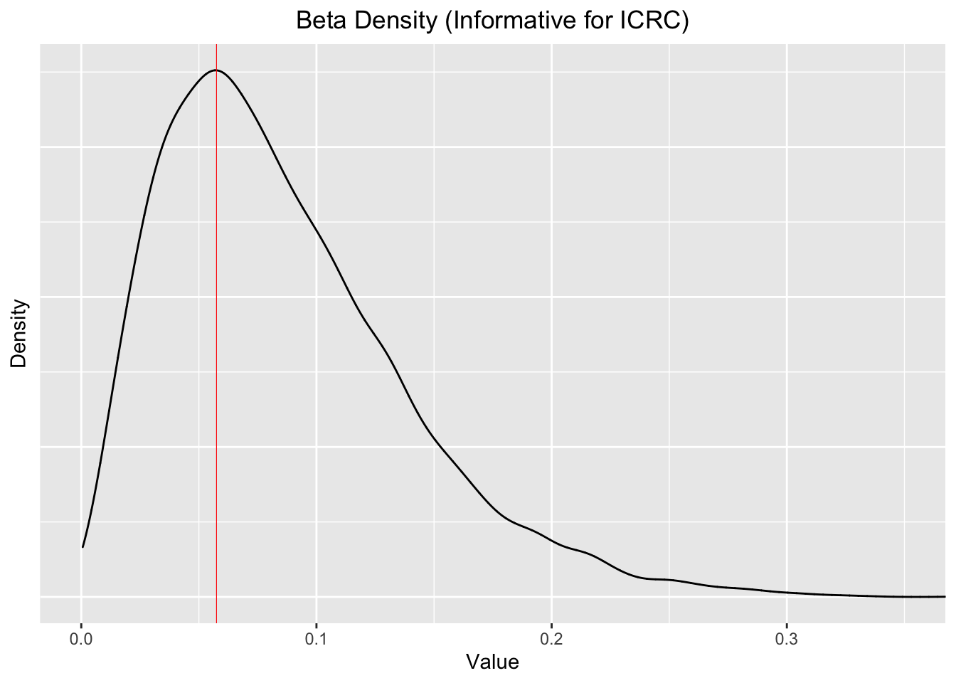
We can consider what this implies for the prior over the absolute and proportional differences in the incidence rates:
beta_inf_compare_i  <- data.frame(control= rbeta(10000, a_e_i, b_e_i), treat = rbeta(10000, a_e_i, b_e_i)) %>%
  as.tibble() %>%
  mutate(
  abs_dif = control-treat,
  scaled_dif = (control-treat)/mean(control)
)

beta_unif_compare_i  <- data.frame(control= rbeta(10000, 1, 1), treat = rbeta(10000, 1, 1)) %>%
  as.tibble() %>%
  mutate(
  abs_dif = control-treat,
  scaled_dif = (control-treat)/mean(control)
)ggplot() +
geom_density(aes(x=scaled_dif, fill = "Informed density"), alpha=0.2, data=beta_inf_compare_i) +
labs(title="Differences as share of mean incidence, comparing two densities") +
geom_density(aes(x=scaled_dif, fill = "Uniform density"), alpha=0.2, data=beta_unif_compare_i) +
theme(plot.title=element_text(hjust=0.5)) +
coord_cartesian(xlim=c(-5, 5)) +
scale_fill_manual(name = "dataset", values = c(Informed = "red", Uniform = "green"))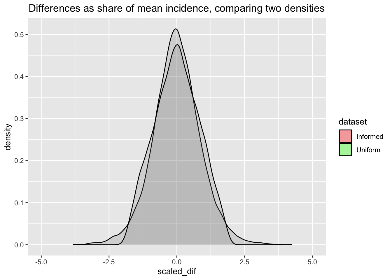
The impact on donation incidence was tightly bounded around a virtual 0 effect. Our posterior here essentially rules out an effect of any substantial magnitude. Even an effect of +/- 2.5% of the base rate (about a tenth of a percentage point impact on actual incidence) is seen as extremely unlikely. The tables below express this more precisely.
Comparison of Posterior Probabilities
bayesian_test_me_by_x <- function(df, colname ="d_impact", outcome="d_don", priora, priorb) {
  g1 <-  sum(df[[colname]] == 0)
  g1pos <-  sum((df[[colname]] == 0)*df[[outcome]])
  g2 <-  sum(df[[colname]] == 1)
  g2pos <-  sum((df[[colname]] == 1)*df[[outcome]])
  bayesian_test_me(g1, g1pos,
                 g2, g2pos,
                 a = priora, b = priorb)
}


icrc_bayes_impact_unif <- bayesian_test_me_by_x(icrc, "d_impact", "d_don", 1, 1)
icrc_bayes_impact_inf <- bayesian_test_me_by_x(icrc, "d_impact", "d_don", a_e_i, b_e_i)


#make this into a function
den_icrc_bayes_impact_unif <- density(icrc_bayes_impact_unif$Differences, bw = 0.15, na.rm = TRUE)

denmax_icrc_bayes_impact_unif <- den_icrc_bayes_impact_unif$x[den_icrc_bayes_impact_unif$y == max(den_icrc_bayes_impact_unif$y)]

den_icrc_bayes_impact_inf <-
density(icrc_bayes_impact_inf$Differences, bw = 0.15, na.rm = TRUE)

denmax_icrc_bayes_impact_inf <- den_icrc_bayes_impact_inf$x[den_icrc_bayes_impact_inf$y == max(den_icrc_bayes_impact_inf$y)]
See details and discussion of this test in our discussion of the Donor Voice trial here
Posterior: Bounds on true difference
(
bounds_icrc <- data.frame(
        Prior = c('Uniform','' , 'Informative',''),
        `Base rate` = c(mu_i)*100,
        MAP = c(op(denmax_icrc_bayes_impact_unif*100), "", op(denmax_icrc_bayes_impact_inf*100),""),
        Bound = c(rep(c("lower","upper"),2)),
        `Dfc. 99pct CI` = c(icrc_bayes_impact_unif$`99LB`, icrc_bayes_impact_unif$`99UB`, icrc_bayes_impact_inf$`99LB`,  icrc_bayes_impact_inf$`99UB`)*100,
        `Dfc. 95pct CI` = c(icrc_bayes_impact_unif$`95LB`, icrc_bayes_impact_unif$`95UB`, icrc_bayes_impact_inf$`95LB`,  icrc_bayes_impact_inf$`95UB`)*100,
        `Dfc. 90pct CI` = c(icrc_bayes_impact_unif$`90LB`, icrc_bayes_impact_unif$`90UB`, icrc_bayes_impact_inf$`90LB`,  icrc_bayes_impact_inf$`90UB`)*100,
 `Dfc. 80pct CI` = c(icrc_bayes_impact_unif$`80LB`, icrc_bayes_impact_unif$`80UB`, icrc_bayes_impact_inf$`80LB`,  icrc_bayes_impact_inf$`80UB`)*100
      ) %>%
  as_tibble() %>%
  .kable(digits=3, caption= "Incidence per 100: Base rate, and bounds (and MAP) on difference by treatment") %>%
  .kable_styling()
)| Prior | Base.rate | MAP | Bound | Dfc..99pct.CI | Dfc..95pct.CI | Dfc..90pct.CI | Dfc..80pct.CI |
|---|---|---|---|---|---|---|---|
| Uniform | 5.217 | 0.0878 | lower | -0.248 | -0.181 | -0.147 | -0.107 |
| 5.217 | upper | 0.310 | 0.243 | 0.208 | 0.168 | ||
| Informative | 5.217 | 0.115 | lower | -0.249 | -0.181 | -0.147 | -0.107 |
| 5.217 | upper | 0.311 | 0.243 | 0.208 | 0.168 |
The table above gives the Bayesian ‘maximum a posteriori’ estimates, and 99, 95, 90, and 80 percent bounds on credible intervals for (differences in) donation incidence. All figures are given ‘per 100’ individuals. We give this both under a completely flat prior (over the baseline incidence rate), and under the informative prior described above. The results are similar for either prior, and bound the effect very tightly around zero. Even under the widest (99 percent) bound, the more extreme bound on the difference is less than ten percent of the base rate of donation (which is 5.22 per 100 individuals.)
#icrc_bayes_impact_unif[!names(icrc_bayes_impact_unif)=="Differences"]

# #forestplot_icrc_ip <- ggplot() +
#   aes(x=value, y=`Credible Intervals`) +
#   geom_point(colour="#4271AE") +
#   geom_line(colour="#4271AE") +
#   facet_grid(rows=vars(Experiment), labeller = label_wrap_gen(multi_line=TRUE, width=2)) +
#   theme(panel.spacing=unit(1,"lines"),plot.title=element_text(hjust=0.5)) +
#   geom_vline(xintercept = 0,size=0.25) +
#   geom_vline(data=forestTableInf$forest_table2, aes(xintercept = `Base rate (conv. per 10k)`, colour = "`Base rate (conv. per 10k)`"),size=0.25 , linetype = "dashed") +
#   geom_vline(data=forestTableInf$forest_table2, aes(xintercept = `MAP Estimate per 10000`, colour = "MAP Estimate"),size=0.25, linetype = "dashed") +
#   labs(x="Delta") +
#   xlim(-10,30) +
#   ggtitle("Credible Intervals by Subset: Informative prior") +
#   scale_colour_manual(name = "Key", values = c("`Base rate (conv. per 10k)`" = "darkblue", "MAP Estimate" = "darkred"))