In December 2021, TLYCS ran a YouTube advertising campaign in single city, involving ‘donation advice’. The top 10% household income households were targeted with (one of) three categories of videos. One of the ultimate goals was to get households to sign up for a ‘concierge’ personal donor advising service.
There were very few signups for the concierge advising service. (About 16 in December 2021 , only 1 from Portland.)
We consider a ‘difference in difference’, to compare the year-on-year changes in visits to TLYCS during this period for Portland vs other comparison cities.
This comparison yields a ‘middle estimate cost’ of $37.7 per additional visitor to the site. This seems relatively expensive. We could look into this further to build a more careful model and consider statistical bounds, if such work is warranted.
5.2 Capturing data
Google Analytics capture
I (David Reinstein) did a manual ‘create report and download’ in TLYCS’s Google Analytics, basically as described here.
The Google Analytics report and it’s parameters can be accessed here, if you have access.
Google Analytics report: parameters and data storage
Report:
3-31 December 2021 vs prior year, same dates
All North American cities with 1 or more user
Counts: Users, sessions, certain types of conversions (see below)
I downloaded this as an Excel spreadsheet to the private eamt_actual_data repo:
# Re-labels the 'correct' Portland (we think), as it's a common city name.^[And there are two other 'Portlands', each with a small number of sessions]tl21 %>%filter(City=="Portland") %>% dplyr::select(City, year, Users, pop2022, pop_gt250k) %>%.kable() %>% .kable_styling
City
year
Users
pop2022
pop_gt250k
Portland
2,021
1
666,453
TRUE
Portland
2,020
0
666,453
TRUE
Portland
2,021
8
666,453
TRUE
Portland
2,020
6
666,453
TRUE
Portland
2,021
306
666,453
TRUE
Portland
2,020
144
666,453
TRUE
relable portland
#Presumably the largest one is Portland, Oregon, and we'll re-label it as such.tl21 <- tl21 %>%mutate(City =case_when(City=="Portland"& Users>20~"Portland_OR", City=="Portland"~"Other_Portland",TRUE~ City) )
tlag <-function(x, n = 1L, time) { index <-match(time - n, time, incomparables =NA) x[index]}tl21 <- tl21 %>%group_by(City) %>%mutate(lag_users =tlag(Users, 1, time = year),diff_users = Users-lag_users,prop_diff_users = diff_users/lag_users ) %>%ungroup()
5.4 Casual/simple ‘uptick’ analysis
Below, for the comparable periods in 2020 and 2021, we give…
…the total numbers of cities in the sample, the share with a positive number of user clicks, and the mean, median, 80th quantile, and standard deviation of the number of clicks.
… For a few subsets
… First for unique user visits, and then for total numbers of sessions.
tabs of session by year
tl21 %>%sumtab(Users, year, caption="All N. Amer. cities")
All N. Amer. cities
year
N
share > 0
Mean
Median
P80
Std.dev.
2020
3006
0.6
9.38
1
4
(296.34)
2021
3006
1.0
13.48
2
4
(425.33)
tabs of session by year
tl21 %>%filter(!City=="Portland_OR") %>%sumtab(Users, year, caption="N. Amer. Cities other than Portland")
N. Amer. Cities other than Portland
year
N
share > 0
Mean
Median
P80
Std.dev.
2020
3004
0.6
3.94
1
4
(21.01)
2021
3004
1.0
5.64
2
4
(30.79)
tabs of session by year
tl21 %>%filter(pop2022>250000) %>%sumtab(Users, year, caption="All N. Amer. Cities with pop. > 250k") #Fix -- filter on over 20 users for 2020 ONLY]
All N. Amer. Cities with pop. > 250k
year
N
share > 0
Mean
Median
P80
Std.dev.
2020
92
0.848
47.46
17.0
47.0
(99.21)
2021
92
1.000
70.04
19.5
80.2
(147.88)
tabs of session by year
tl21 %>%sumtab(Sessions, year, caption="Sessions by year, all")
Sessions by year, all
year
N
share > 0
Mean
Median
P80
Std.dev.
2020
3006
0.6
11.75
1
4
(370.61)
2021
3006
1.0
16.80
2
5
(528.67)
Note that all measures generally show an increase from year to year.
lower bound on cost of $13.07 per user ($10.28 per visit) if ‘all visits were generated by the ad’, and
a somewhat more reasonable $24.69 cost per user if Portland was the ‘same as last year’. But it seems most reasonable to allow Portland to have similar trends as other cities.
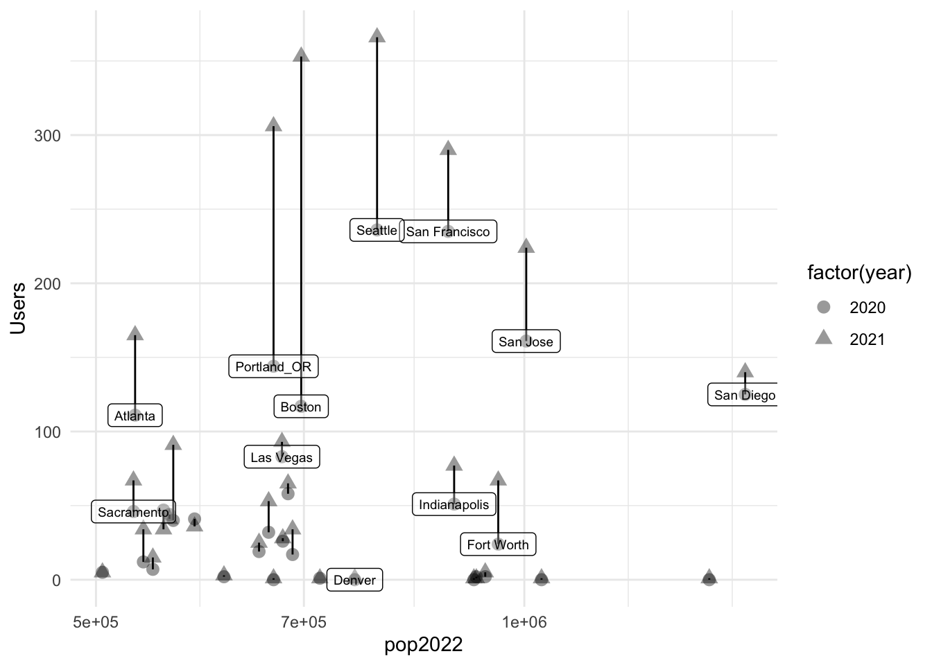
Difference in Differences comparison to other cities
Guiding assumptions:
the cities used are fairly representative
‘uptick as a percentage’ is unrelated to city size/visits last year
all the cities in the comparison group are ‘informative to the counterfactual’ in proportion to their total number of sessions.4
Thus
112.5% visits uptick (Year on Year) for Portland in 2020
For ‘all North American cities other than Portland (with greater than 250,000 people )’:
The average is 46.5 users in the 2020 period and 64.5 users in the 2021 period, an uptick of 64.5 - 46.5)/46.5 = about 38.8%. 5
38.8% uptick \(\times\) 144 = 55.9 ‘counterfactual uptick’ in users for Portland
162 -55.9 = 106 ‘uptick relative to counterfactual’
The above comparisons are crude and have limitations:
All cities are weighted equally, no matter their size or similarity to Portland
Some year-to-year idiosynchratic variation may be unrelated to trends or to the trial. We have not ‘quantified this uncertainty’
If we want a more precise estimate and careful CIs6 we can build an explicit model and simulation. But I want to know the value of precision here before I dig deeper.
Note: the code below reads directly from the folder structure and is thus not portable. Ideally, we would modify this to read it in directly from the private Github repo for those with access.↩︎
Downloaded from this link accessed on 17 Mar 2022; we add the largest-15 Canadian cities as well (hand-input)↩︎
The present very simple section is hand-input for now…↩︎
I’m waving the hands a bit here; this is not precise.↩︎
This is very similar to the result if we look at all cities which has an uptick of 43.1%↩︎
confidence, credible or ‘consistent intervals’, depending on model and terminology↩︎
Source Code
# TLYCS Portland trial: Brief report**Background, data input, brief report**```{r, include=FALSE}library(here)library(pacman)p_load(dplyr, plotly, install =FALSE)source(here("code", "shared_packages_code.R"))```## The trialIn December 2021, TLYCS ran a YouTube advertising campaign in single city, involving 'donation advice'. The top 10% household income households were targeted with (one of) three categories of videos. One of the ultimate goals was to get households to sign up for a 'concierge' personal donor advising service.The details are presented in our gitbook [HERE](https://effective-giving-marketing.gitbook.io/untitled/partners-contexts-trials/the-life-you-can-save-tlycs/advisor-signup-portland)### Quick takeaways {-}There were very few signups for the concierge advising service. (About 16 in December 2021 , only 1 from Portland.)We consider a 'difference in difference', to compare the year-on-year changes in visits to TLYCS during this period for Portland vs other comparison cities.This comparison yields a 'middle estimate cost' of \$37.7 per additional visitor to the site. This seems relatively expensive. We could look into this further to build a more careful model and consider statistical bounds, if such work is warranted.## Capturing data::: {.callout-note collapse="true"}## Google Analytics captureI (David Reinstein) did a manual 'create report and download' in TLYCS's Google Analytics, basically as described [here](https://effective-giving-marketing.gitbook.io/untitled/marketing-and-testing-opportunities-tools-tips/collecting-data-trial-outcomes/google-analytics-interface). The Google Analytics report and it's parameters can be accessed [here](https://analytics.google.com/analytics/web/#/my-reports/mmZsQ-HMSbCwiG5hjQhWhQ/a10056556w22050110p185278310/_u.date00=20211203&_u.date01=20211231&_u.date10=20201203&_u.date11=20201231&197-table.advFilter=%5B%5B1,%22analytics.totalVisitors%22,%22GT%22,%220%22,0%5D%5D&197-table.plotKeys=%5B%5D&197-table.rowCount=5000&197-table-dataTable.sortColumnName=analytics.totalVisitors&197-table-dataTable.sortDescending=false&197-graphOptions.primaryConcept=analytics.totalVisitors&197-graphOptions.compareConcept=analytics.visits), if you have access.::: ::: {.callout-note collapse="true"}## Google Analytics report: parameters and data storageReport:- 3-31 December 2021 vs prior year, same dates- All North American cities with 1 or more user- Counts: Users, sessions, certain types of conversions (see below)I downloaded this as an Excel spreadsheet to the private `eamt_actual_data` repo:`eamt_actual_data/tlycs/tlycs_dec_2021_vs_2020_by_city_n_america.xlsx`<!-- (This is gitignored so it won't be 'committed' to our repo, at least for now) -->::: ## Input and clean data^[Note: the code below reads directly from the folder structure and is thus not portable. Ideally, we would modify this to read it in directly from the private Github repo for those with access.]```{r}#| label: read_tlycs#| code-summary: "Reading TLYCS trial data"#tl21 <- read_excel(here::here("data_do_not_commit", "tlycs", "tlycs_dec_2021_vs_2020_by_city_n_america.xlsx"), sheet = "Dataset1") #this should have worked?#tl21 <- readxl::read_excel("~/githubs/eamt_actual_data/tlycs/tlycs_dec_2021_vs_2020_by_city_n_america.xlsx", sheet = "Dataset1")tl21 <- readxl::read_excel(here::here("tlycs_portland_trial_2021", "tlycs_dec_2021_vs_2020_by_city_n_america.xlsx"), sheet ="Dataset1") %>% dplyr::as_tibble()```We add companion data on US city sizes.^[Downloaded from [this link](https://worldpopulationreview.com/us-cities) accessed on 17 Mar 2022; we add the largest-15 Canadian cities as well (hand-input)]```{r }#| label: us_cities_pop#| code-summary: "input cities data"us_cities_pop <-read.csv(here::here("tlycs_portland_trial_2021", "uscities_pop.csv")) %>% dplyr::select(name, rank, usps, pop2022) %>%mutate(name =if_else(name=="New York City", "New York", name)) %>%as_tibble()tl21 <-left_join( tl21, us_cities_pop,by =c("City"="name") ) %>%mutate(pop_gt250k = pop2022>250000|str_det(City, "Windsor|Oshawa|Halifax|Victoria|Kitchener|Hamilton|Quebec|Winnipeg|Ottawa|Edmonton|Calgary|Vancouver|Montreal|Toronto") ) %>% dplyr::select(City, `Date Range`, Users, pop2022, pop_gt250k, everything())```::: {.callout-note collapse="true"}## More codingBelow, we:- Choose the 'largest Portland' as this must be Portland, OR- Drop other city duplicates to enable lagging/leading more easily- Creates lags and 'differences across years' features.::: ```{r}#| label: year_feature#| code-summary: "Create 'year' feature"tl21 <- tl21 %>%mutate(year =case_when(str_detect(`Date Range`, "2021") ==TRUE~2021,str_detect(`Date Range`, "2020") ==TRUE~2020 ))``````{r}#| label: table_portland#| code-summary: "Table of 'Portland' cities"# Re-labels the 'correct' Portland (we think), as it's a common city name.^[And there are two other 'Portlands', each with a small number of sessions]tl21 %>%filter(City=="Portland") %>% dplyr::select(City, year, Users, pop2022, pop_gt250k) %>%.kable() %>% .kable_styling``````{r }#| label: relable_portland#| code-summary: "relable portland"#Presumably the largest one is Portland, Oregon, and we'll re-label it as such.tl21 <- tl21 %>%mutate(City =case_when(City=="Portland"& Users>20~"Portland_OR", City=="Portland"~"Other_Portland",TRUE~ City) )``````{r }#| label: drop_dup_cities#| code-summary: "drop_dup_cities"tl21 <- tl21 %>%rowwise() %>%mutate(key =paste(sort(c(City, year)), collapse="")) %>%distinct(key, .keep_all=T) %>% dplyr::select(-key) %>% ungroup``````{r}#| label: lag_stuff#| code-summary: "Create lag and difference features"tlag <-function(x, n = 1L, time) { index <-match(time - n, time, incomparables =NA) x[index]}tl21 <- tl21 %>%group_by(City) %>%mutate(lag_users =tlag(Users, 1, time = year),diff_users = Users-lag_users,prop_diff_users = diff_users/lag_users ) %>%ungroup()```<!-- ## Exploratory analysis; todo -->## Casual/simple 'uptick' analysisBelow, for the comparable periods in 2020 and 2021, we give... ...the total numbers of cities in the sample, the share with a positive number of user clicks, and the mean, median, 80th quantile, and standard deviation of the number of clicks.... For a few subsets... First for unique user visits, and then for total numbers of sessions.```{r}#| label: sumtabs_users#| code-summary: "tabs of session by year"tl21 %>%sumtab(Users, year, caption="All N. Amer. cities")tl21 %>%filter(!City=="Portland_OR") %>%sumtab(Users, year, caption="N. Amer. Cities other than Portland")tl21 %>%filter(pop2022>250000) %>%sumtab(Users, year, caption="All N. Amer. Cities with pop. > 250k") #Fix -- filter on over 20 users for 2020 ONLY]tl21 %>%sumtab(Sessions, year, caption="Sessions by year, all")```Note that all measures generally show an increase from year to year.```{r}#| label: or_v_non_or_uptick#| code-summary: "Upticks for Oregon, other"OR_users_21 <- tl21 %>% dplyr::filter(City=="Portland_OR"& year==2021) %>% dplyr::select('Users') %>%pull()OR_users_20 <- tl21 %>% dplyr::filter(City=="Portland_OR"& year==2020) %>% dplyr::select('Users') %>%pull()OR_uptick <- OR_users_21 - OR_users_20nonOR <- tl21 %>% dplyr::filter(City!="Portland_OR") %>% dplyr::select('Users', year)nonOR_gt250k <- tl21 %>% dplyr::filter(pop_gt250k==TRUE) %>% dplyr::select('Users', year)nonOR_users_21 <-mean(nonOR$Users[nonOR$year==2021])nonOR_users_20 <-mean(nonOR$Users[nonOR$year==2020])nonOR_uptick <- (nonOR_users_21 - nonOR_users_20)/nonOR_users_20nonOR_gt250k_users_21 <-mean(nonOR_gt250k$Users[nonOR_gt250k$year==2021])nonOR_gt250k_users_20 <-mean(nonOR_gt250k$Users[nonOR_gt250k$year==2020])nonOR_gt250k_uptick <- (nonOR_gt250k_users_21 - nonOR_gt250k_users_20)/nonOR_gt250k_users_20```### Bounding : Maximum impact/minimum cost (subject to random variation) {-}(This duplicates the <!-- (todo: integrate in) update --> hand-calculated results in Gitbook [HERE](https://app.gitbook.com/o/-MfFk4CTSGwVOPkwnRgx/s/-Mf8cHxdwePMZXRTKnEE/contexts-and-environments-for-testing/tlycs/advisor-signup-portland/results-first-pass))^[The present very simple section is hand-input for now...]We have a....- lower bound on cost of \$13.07 per user (\$10.28 per visit) if 'all visits were generated by the ad', and - a somewhat more reasonable \$24.69 cost per user if Portland was the 'same as last year'. But it seems most reasonable to allow Portland to have similar trends as other cities.### Difference in Differences comparison to other cities {-}Guiding assumptions:- the cities used are fairly representative- 'uptick as a percentage' is unrelated to city size/visits last year- all the cities in the comparison group are 'informative to the counterfactual' in proportion to their total number of sessions.^[I'm waving the hands a bit here; this is not precise.]\*Thus*`r 100*(OR_users_21 - OR_users_20)/OR_users_20`% visits uptick (Year on Year) for Portland in 2020For 'all North American cities other than Portland (with greater than 250,000 people )':The average is `r op(mean(nonOR_gt250k$Users[nonOR_gt250k$year==2020]))` users in the 2020 period and `r op(mean(nonOR_gt250k$Users[nonOR_gt250k$year==2021]))` users in the 2021 period, an uptick of `r op(nonOR_gt250k_users_21)`- `r op(nonOR_gt250k_users_20)`)/`r op(nonOR_gt250k_users_20)` = about `r op(100*nonOR_gt250k_uptick)`%.^[This is very similar to the result if we look at all cities which has an uptick of `r op(100*nonOR_uptick)`%]`r op(100*nonOR_gt250k_uptick)`% uptick $\times$ `r OR_users_20` = `r op(nonOR_gt250k_uptick*OR_users_20)` 'counterfactual uptick' in users for Portland`r OR_users_21 - OR_users_20` -`r op(nonOR_gt250k_uptick*OR_users_20)` = `r op(OR_users_21 - OR_users_20 - nonOR_gt250k_uptick*OR_users_20)` 'uptick relative to counterfactual'```{r}or_uptick_vs_cfl_gt250 <- OR_users_21 - OR_users_20 - nonOR_gt250k_uptick*OR_users_20```USD 4000 /`r op(or_uptick_vs_cfl_gt250)` = \$ `r op(4000/or_uptick_vs_cfl_gt250)` cost per userThis seems realistic at a first-pass.\### Plotting the 'difference in difference' {-}Scatterplot of unique users by city, both time periods, US cities with 500k-1.5mill population, Portland highlighted```{r }#| label: users_by_year#| code-summary: "users_by_year"( users_by_year <- tl21 %>%filter(pop2022 >=500000& pop2022 <1500000) %>%ggplot() +aes(x = pop2022, y = Users, label = City) +geom_point(aes(shape =factor(year)), size=3, alpha=0.4) +geom_path(aes(group = City)) +geom_label(data =subset(tl21, City %in%c('Portland_OR','Boston','Seattle', 'San Francisco', 'Atlanta', 'San Diego', 'Indianapolis', 'Fort Worth', 'Sacramento', 'Denver', 'San Jose', 'Las Vegas') & year==2020), alpha =0.3, size =2.5) +scale_x_continuous(trans='log10') +theme_minimal())#users_by_year %>% plotly::ggplotly()```Plotting increases in users by population...```{r, warning=FALSE}#| label: increase_by_size#| code-summary: "increase_by_size"( increase_by_size <- tl21 %>%filter(pop2022 >=500000& pop2022 <1500000& year==2021) %>%ggplot() +aes(x = pop2022, y = diff_users, label = City) +geom_point(size=3, alpha=0.4) +geom_label(data =subset(tl21, City %in%c('Portland_OR','Boston','Seattle', 'San Francisco', 'Atlanta', 'San Diego', 'Indianapolis', 'Fort Worth', 'Sacramento', 'Denver', 'San Jose', 'Las Vegas')), alpha =0.3, size =2.5) +scale_x_continuous(trans='log10') +theme_minimal())```Plotting proportional increases in users by 2020 users...```{r}( prop_increase_by_size <- tl21 %>%filter(pop2022 >=500000& pop2022 <1500000& year==2021& lag_users>0) %>%ggplot() +aes(x = lag_users, y = prop_diff_users, label = City) +geom_point(size=3, alpha=0.4) +geom_smooth(method='lm') +geom_text(hjust=0, vjust=0, alpha=.5) +scale_x_continuous(trans='log10') +theme_minimal() +ggtitle("Mid-sized cities, proportional changes") +xlab("Users in 2020") +ylab("Proportional change in users"))```## Next steps, if warrantedThe above comparisons are crude and have limitations:- All cities are weighted equally, no matter their size or similarity to Portland- Some year-to-year idiosynchratic variation may be unrelated to trends or to the trial. We have not 'quantified this uncertainty'If we want a more precise estimate and careful CIs^[confidence, credible or 'consistent intervals', depending on model and terminology] we can build an explicit model and simulation. But I want to know the value of precision here before I dig deeper.