Installing BiocManager [1.30.20] ...
OK [linked cache]1 Giving What We Can: Giving guides
Note
This chapter aligns with, and supplements the EA Forum post “Marketing messages trial for GWWC Giving Guide Campaign”
1.1 Quick overview
Context: Facebook ads on a range of audiences
… [with text and rich content promoting effective giving and a “giving guide” – links people to a Giving What We Can page asking for their email in exchange for the guide]
Objective: Test distinct approaches to messaging, aiming to get people to download our Giving Guide. (Previously called “emotional and factual” approaches; basically these were “Charity research facts” vs. “cause focus”)
Process and further goals: GWWC worked with a creative agency to develop a set of animated video ads wiht differing texts. This work is also informative about costs and the ‘value of targeting’ in this context. Note these ads had several ‘versions’ during the campaign (see ‘Test 1 - Test 4’).
Key findings:
The cost of an email address acquired via a Facebook campaign during Giving Season was as low as $8.00 across campaigns but could be lower with more targeting.
“Only 3% of people give effectively,” seems to be an effective message for generating link clicks and email addresses vs. the other messages.
Lookalike and animal rights audiences seem the most promising audiences.
Demographics are not very predictive on a per-$ basis.
Key caveats
Specificity and interpretation: All comparisons are not for ‘audiences of similar composition’ but for ‘the best audience Facebook could find to show the ads, within each group, according to its algorithm’. Thus differences in performance may combine ‘better targeting’ with ‘better performance on the targeted group’. See our detailed discussion HERE.
I.e., we can make statements about “what works better on Facebook in this context and maybe similar contexts”
but not about “which audience, as defined, is more receptive” (as the targeting within each audience may differ in unobserved ways),
nor about “which message works better on a particular comparable audience” (for the same reason)
Outcome is ‘click to download the giving guide’.
Code: Import raw data for descriptions
#importing for dynamic input of descriptions below

#Todo: get direct import working: See https://cran.r-project.org/web/packages/rfacebookstat/rfacebookstat.pdf

raw_data_path <- list("gwwc", "gg_raw_data_shareable")

mini_clean <- function(df){
  df %>%
    as_tibble() %>%
  janitor::clean_names() %>%
  janitor::remove_empty() %>% # removes empty rows and columns, here `unique_link_clicks`
    janitor::remove_constant()
    }

gg_campaign_by_ad_by_text <- read_csv(here(raw_data_path, "gg_campaign_by_ad_by_text.csv"), show_col_types=FALSE) %>%
  dplyr::select(-"Campaign name...4") %>% #duplicate columns?
 mini_clean
1.2 The trial
Context: Facebook advertisements with a range of audiences/filters1
Effective Giving Guide Lead Generation campaign … ran late November 2021 - January 2022. The objective of this campaign was to see whether a factual [‘who researches giving’ or ‘magnitude of impact differences’] or cause-led approach was more cost-effective at getting people to fill out a form and give us their email in order to download our Effective Giving Guide.
The page they were directed to, “Learn how to give more effectively” allowed you to download the guide only after leaving your email.
Treatments (text \(\times\) video)
There were two dimensions of treatment content:2
- The texts displayed above the videos
Texts
Bigger difference next year: Want to make a bigger difference next year? Start with our Effective Giving Guide and learn how to make a remarkable impact just by carefully choosing the charities you give to.
100x impact: Did you know that the best charities can have a 100x greater impact? Download our free Effective Giving Guide for the best tips on doing the most good this holiday season.
6000 people: Giving What We Can has helped 6,000+ people make a bigger impact on the causes they care about most. Download our free guide and learn how you can do the same.
Cause list: Whether we’re moved by animal welfare, the climate crisis, or worldwide humanitarian efforts, our community is united by one thing: making the biggest impact we can. Make a bigger difference in the world through charitable giving. Start by downloading our Effective Giving Guide. You’ll learn how to approach charity research and smart giving. And be sure to share it with others who care about making a greater impact on the causes closest to their hearts.
Learn: Use our free guide to learn how to make a bigger impact on the causes you care about most.
Only 3% research: Only 3% of donors give based on charity effectiveness yet the best charities can be 100x more impactful. That’s incredible! Check out the Effective Giving Guide 2021. It’ll help you find the most impactful charities across a range of causes.
Overwhelming: It can be overwhelming with so many problems in the world. Fortunately, we can do a lot to help, if we give effectively. Check out the Effective Giving Guide 2021. It’ll help you find the most impactful charities across a range of causes.
Full text: exported from data set
Giving What We Can has helped 6,000+ people make a bigger impact on the causes they care about most. Download our free guide and learn how you can do the same., It can be overwhelming with so many problems in the world. Fortunately, we can do a lot to help, if we give effectively.
Check out the Effective Giving Guide 2021. It’ll help you find the most impactful charities across a range of causes., Use our free guide to learn how to make a bigger impact on the causes you care about most., Want to make a bigger difference next year? Start with our Effective Giving Guide and learn how to make a remarkable impact just by carefully choosing the charities you give to., Whether we’re moved by animal welfare, the climate crisis, or worldwide humanitarian efforts, our community is united by one thing: making the biggest impact we can.
Make a bigger difference in the world through charitable giving. Start by downloading our Effective Giving Guide. You’ll learn how to approach charity research and smart giving. And be sure to share it with others who care about making a greater impact on the causes closest to their hearts., Did you know that the best charities can have a 100x greater impact? Download our free Effective Giving Guide for the best tips on doing the most good this holiday season., Only 3% of donors give based on charity effectiveness yet the best charities can be 100x more impactful. That’s incredible!
Check out the Effective Giving Guide 2021. It’ll help you find the most impactful charities across a range of causes.
- The Video ads theme and content
“Facts”
Charity research facts short video (8 seconds): Only 3% of donors research charity effectiveness, yet the best charities can 100x your impact, learn how to give effectively
Charity research facts long video (22 seconds): Trivial things we search (shows someone searching how to do Gangnam style), things we should research (shows someone searching how to donate effectively), only 3% of donors research charity effectiveness, yet the best charities can 100x your impact, learn how to give effectively. Slower paced music compared to the short video and cause videos.
“Cause focus”
Climate change (15 seconds): Care about climate change? You don’t have to renounce all your possessions, But you could give to effective environmental charities, Learn how to maximize your charitable impact, Download the Effective Giving Guide
Animal welfare (16 seconds): Care about animals? You don’t have to adopt 100 cats, But you could give to effective animal charities, Learn how to maximize your charitable impact, Download the Effective Giving Guide
Poverty (16 seconds): Want to help reduce global poverty? You don’t have to build a village, But you could give to effective global development charities, Learn how to maximize your charitable impact, Download the Effective Giving Guide
Arguments, rich content from “Brand Video”
- Brand Video (1 min 22 seconds): Animated and voiceover video that explains how GWWC can help maximize charitable impact (support, community, and information) and the problems GWWC addresses (good intentions don’t always produce the desired outcomes, there are millions of charities that have varying degrees of impact and some can even cause harm). CTA: Check out givingwhatwecan.org to learn how you can become an effective giver.
Further detail, links
Notes from the trial description
“In the original version of our test, we had 1 video for the factual appeal and 3 videos for the cause led approach - 1 for global health and development, 1 for animal welfare and 1 for climate change.”
“We targeted our ads to audiences we thought were likely to engage based on their interests and demographics, and targeted the cause led videos to a relevant audience, i.e. climate change message to climate change audience.”
“We also had various text above the videos that were displayed and optimized.”
Details in Gitbook HERE (and embedded below) and Gdoc here
Code
knitr::include_url("https://effective-giving-marketing.gitbook.io/untitled/partner-organizations-and-trials/gwwc/giving-guides-+")Implementation & assignment: key details
Treatment assignment order, dates
The treatment assignment was determined by Facebook’s algorithm. Video content was manipulated across three split tests.
Test 1 (Nov 30, 2021 – Dec 8, 2021, campaigns: “Cause-Led” and “Factual”) displayed either the long factual video or a cause focus video. In the cause focus condition, cause-specific audiences for animal rights, climate change, and poverty (based on their behavior on Facebook) were shown the relevant cause video.
Test 2 (Starting December 8, campaign “Factual V2”?) was the same as Test 1 but used the short factual video instead of the cause-focus videos.
Test 3 (Starting December 23, campaign “Cause-led V3” and “Factual V3” (?)): was the same as Test 2 but had a new version of the videos (with Luke just holding up signs with the words). This test was also restricted to 18-35 (or 18-44) year olds.3
Test 4: (Starting December 23, “Brand Video” and “PPCo”) The Brand Video was displayed in a separate campaign which was tested against another campaign that allowed the algorithm to optimize between the ‘short factual’ and ‘cause focus’ videos (although not allowing each cause-specific audience to see the ads for other cause areas).
In all tests, the text content displayed above the video was determined by Facebook’s algorithm. Balance across variations was determined to equate budgets across split tests; otherwise, according to Facebook’s algorithm. All variation was done at the level of the impression.
The videos were adapted across the trials as we learned. First, we updated the factual video to be shorter for Trial 2, and then we tried videos of Luke holding up signs spelling out the voiceover in Trial 3 for all videos.
1.3 Build: Source data, cleaning
Accessing, downloading, inputting data
See:
https://effective-giving-marketing.gitbook.io/untitled/marketing-and-testing-opportunities-tools-tips/collecting-data-trial-outcomes/facebook-meta-ads-interface
Accessing and bringing down simple results HERE
We import the exported ‘pivot table’ gg_campaign_by_ad_by_text below, as well as the more detailed version, broken down by age range and gender: gg-campaign-by-ad-set-text-age-gender.csv.4
Data structure
The data frame gg_campaign_by_ad_by_text_age_gender has one row per combination of ‘campaign, ad, text, age group, gender’.
Each row represents a combination of the below (with different numbers of ‘reach’ for each row)5
campaign_name: When and and with what funds the ad was launched, I think (?)ad_set: An ad set can specifically tie anad_nameto an audience (I think)ad_name: Which video/media (or collection of optimized videos/media) was shown; note this is paired with ‘which audience’ in it’s label, as there were specific ‘global poverty’, ‘animal welfare’, ‘climate change’, ‘philanthropy’ and ‘retargeting’ audiences- Caveat: The
ad_nameseems to select from a different set of media for optimization depending on whichad_setit is in.6
- Caveat: The
text: Which text was shown along with the videoage(a range of ages)gender(female, male, unknown)
Import raw data
raw_data_path <- list("gwwc", "gg_raw_data_shareable")

#already input above: gg_campaign_by_ad_by_text

#Version allowing demographic breakdown:
gg_campaign_by_ad_by_text_age_gender <- read_csv(here(raw_data_path, "gg-campaign-by-ad-set-text-age-gender.csv"), show_col_types=FALSE) %>%
  #dplyr::select(-"Campaign name...4") %>% #duplicate columns?
 mini_clean()

#Version with information on cause videos shown (even to those in 'general' groups):

gg_video_breakdowns <- read_csv(here(raw_data_path, "gg-image-video-breakdowns.csv"), show_col_types=FALSE)

#capture and remove columns that are the same everywhere
attribution_setting_c <- gg_campaign_by_ad_by_text_age_gender$attribution_setting %>% .[1]
reporting_starts_c <- gg_campaign_by_ad_by_text_age_gender$reporting_starts %>% .[1]
reporting_ends_c <- gg_campaign_by_ad_by_text_age_gender$reporting_ends %>% .[1]

gg_campaign_by_ad_by_text_age_gender  %<>% mini_clean()
gg_video_breakdowns  %<>% mini_clean()

#functions to clean these specific data sets 'gg_campaign_by_ad_by_text_age_gender' and 'gg_campaign_by_ad_by_text':
source(here("gwwc", "giving_guides", "clean_gg_raw_data.R"))

#Many cleaning steps: audience, video_theme, campaign_theme, agetrin; releveling
gg_campaign_by_ad_by_text_age_gender %<>%
  rename_gg() %>%
gg_make_cols() %>%
  text_clean() %>%  # Shorter 'text treatment' column
  dplyr::select(campaign_name, everything(), -campaign_name_1, -campaign_name_7) #campaign_name_7 was the same as campaign_name_1

gg_video_breakdowns %<>%
  rename_gg() %>%
gg_make_cols()

#gg_campaign_by_ad_by_text_age_gender %>% collapse::descr()
Encode video types
gg_video_breakdowns %<>%
  mutate(
    video_theme = case_when(
      str_det(image_video_and_slideshow, "set_1|Animals") ~ "Animal",
      str_det(image_video_and_slideshow, "set_2|Climate") ~ "Climate",
      str_det(image_video_and_slideshow, "set_3|Poverty") ~ "Poverty",
      str_det(image_video_and_slideshow, "Free Effective") & video_theme=="Cause-led (any)" ~ "Poverty",
      str_det(image_video_and_slideshow, "factual_short|Factual Short") ~ "Factual short",
    TRUE ~   video_theme
    ),
    video_theme =  factor(video_theme),
    video_theme = fct_relevel(video_theme, c("Animal", "Climate", "Poverty", "Factual short", "Factual long", "Branded (factual)"))
  )
Export/save data
cleaned_data_path <- list("gwwc", "gg_processed_data")

#export 'cleaned' data for others to play with immediately
write.csv(gg_video_breakdowns, here(cleaned_data_path, "gg_video_breakdowns.csv"), row.names = FALSE)
write.csv(gg_campaign_by_ad_by_text_age_gender, here(cleaned_data_path, "gg_campaign_by_ad_by_text_age_gender.csv"), row.names = FALSE)

write_rds(gg_video_breakdowns, here(cleaned_data_path, "gg_video_breakdowns.Rdata"))
write_rds(gg_campaign_by_ad_by_text_age_gender, here(cleaned_data_path, "gg_campaign_by_ad_by_text_age_gender.Rdata"))
This data is being publicly shared; above, ‘export’ above
This data is clearly not identifying individuals; it involves aggregates based on real or assumed characteristics … there is likely nothing that needs to be hidden here. We are sharing and integrating all the data in this repo, for a complete pipeline.
In the code above, we create several ‘cleaned data’ files for others to access in the linked Github repo (under gwwc.)
You can access the original data referred to above, and/or fork or clone our public Github repository and run the present code if you like.
Previous version of data used … (moved)
We previously used data collapsed (breakdowns) by demography and ad set, into 2 files, which duplicated rows to represent the number of people reached: video breakdown, and text breakdown.csv. We now use the more ‘raw’ minimal version of the data, avoiding duplicating rows where possible.
Below, we also input some of the ‘old version’ of the data, with the duplicated rows, to accommodate the old-format of analysis … this will be removed when we switch over. The code above inputs and builds 2-4 related data frames (tibbles), which were constructed from the collapsed (aggregated) data by multiplying rows according to observation counts. I am not sure where this was done. Once we update the rest we will get rid of this. …
e.g.,
gwwc_vid_results: Observations of emails provided… by video content
This content/input has been moved to eamt_data_analysis/gwwc/giving_guides/archive_erin/erin_plots_stats_gg.qmd, at least for now
1.4 Descriptives
1.4.1 Implemented treatments, ‘reach’ {-reach}
First we illustrate ‘where, when, and to whom’ the different campaigns and treatments were shown (‘people reached’ on Facebook).
We use ‘reach’ as our metric throughout’; essentially ‘unique impressions’
According to Facebook (https://business.facebook.com/adsmanager/ accessed 5 Aug 2022), reach is:
The number of people who saw your ads at least once. Reach is different from impressions, which may include multiple views of your ads by the same people.
In all of our figures below we use the reach outcome rather than the ‘impressions’ outcome, although we sometimes refer to it as ‘impressions’, because it is a clearer way of describing it.
The sequential campaigns involved different sets of videos.
Code
(
  reach_campaign_theme <- gg_video_breakdowns %>%
  dplyr::select(campaign_name, video_theme, reach) %>%
   uncount(weights = .$reach) %>%
    dplyr::select(-reach) %>%
   tabyl(campaign_name, video_theme) %>%
    dplyr::select(campaign_name, Animal, Climate, Poverty, everything()) %>%
  .kable(caption = "Campaign names and video themes: unique impressions") %>%
  .kable_styling()
)| campaign_name | Animal | Climate | Poverty | Factual short | Factual long | Branded (factual) |
|---|---|---|---|---|---|---|
| Branded | 0 | 0 | 0 | 0 | 0 | 56,694 |
| Giving Guide 2021 - Cause-led | 81,298 | 5,272 | 33,027 | 0 | 0 | 0 |
| Giving Guide 2021 – Cause-led V3 | 37,680 | 3,882 | 60,346 | 0 | 0 | 0 |
| Giving Guide 2021 – Factual | 0 | 0 | 0 | 2,333 | 25,316 | 0 |
| Giving Guide 2021 – Factual V2 | 0 | 0 | 0 | 103,329 | 0 | 0 |
| Giving Guide 2021 – Factual V3 | 0 | 0 | 0 | 112,203 | 0 | 0 |
| Giving Guide 2021 – PPCo Creatives | 23,037 | 23,238 | 2,383 | 62,116 | 0 | 0 |
Code
reach_campaign_audience <- gg_campaign_by_ad_by_text_age_gender %>% #created but not shown for now
  dplyr::select(campaign_name, audience, reach) %>%
   uncount(weights = .$reach) %>%
    dplyr::select(-reach) %>%
   tabyl(campaign_name, audience) %>%
  .kable(caption = "Campaign names and audiences: unique impressions") %>%
  .kable_styling()
These videos had different versions
Code
(
  versions_of_videos <- gg_campaign_by_ad_by_text_age_gender %>%
  dplyr::select(video_theme, version, reach) %>%
   uncount(weights = .$reach) %>%
    dplyr::select(-reach) %>%
   table %>%
  .kable(caption = "Versions of videos: unique impressions") %>%
  .kable_styling()
)| V1 | V2 - factual shortened | V3 - sometimes Luke | Video/creatives | |
|---|---|---|---|---|
| Animal | 40,852 | 0 | 20,593 | 0 |
| Branded (factual) | 0 | 0 | 0 | 66,393 |
| Cause-led (any) | 79,624 | 0 | 75,570 | 117,888 |
| Climate | 1,779 | 0 | 339 | 0 |
| Factual long | 29,589 | 0 | 0 | 0 |
| Factual short | 0 | 109,262 | 120,244 | 0 |
| Poverty | 7,906 | 0 | 12,017 | 0 |
#### Which videos were shown to which audiences? {-which_videos}
Some audiences were profiled as being associated with a certain cause (through their Facebook interests or activities): in ‘cause-focused’ campaigns they were shown videos for their profiled cause. In campaigns that were not cause-focused, they were shown general interest videos. However, those associated with one cause were never shown videos for other causes.
Audiences not associated with a cause included the ‘General’ audience, the Philanthropy (interested in charity) audience, a GWWC ‘Lookalike’ audience, and a Retargeted audience: these audiences were shown either the more general-interest videos or particular cause videos.7 This is illustrated in the table below.
Code
video_levels <- c("Animal", "Climate", "Poverty", "Factual short",  "Factual long", "Branded (Factual)", "Total")

audience_levels <- c("Animal", "Climate", "Global Poverty", "Philanthropy", "General audience", "Lookalikes", "Retargeting")


adorn_opts <- function(df) {
  df %>%
    adorn_percentages("all") %>%
    adorn_totals(where = c("row", "col")) %>%
    adorn_pct_formatting(digits = 2)
}

(
reach_video_audience <- gg_video_breakdowns %>%
    dplyr::select(video_theme, audience, reach) %>%
    uncount(weights = .$reach) %>%
    dplyr::select(-reach) %>%
    tabyl(audience, video_theme) %>%
    adorn_opts() %>%
    dplyr::select(audience, Animal, Climate,Poverty, everything()) %>%
   mutate(audience =  factor(audience, levels = audience_levels)) %>%
  arrange(audience)  %>%
    .kable(caption = "Video themes (columns) by audience (rows): share of unique impressions", digits=3) %>%
  .kable_styling()


)| audience | Animal | Climate | Poverty | Factual short | Factual long | Branded (factual) | Total |
|---|---|---|---|---|---|---|---|
| Animal | 9.77% | 0.00% | 0.00% | 11.84% | 1.22% | 0.95% | 23.78% |
| Climate | 0.00% | 1.80% | 0.00% | 12.53% | 1.19% | 2.26% | 17.78% |
| Global Poverty | 0.00% | 0.00% | 3.04% | 4.88% | 0.64% | 1.05% | 9.60% |
| Philanthropy | 10.02% | 1.88% | 9.26% | 8.19% | 0.88% | 1.88% | 32.11% |
| General audience | 1.35% | 0.98% | 0.18% | 2.11% | 0.00% | 2.67% | 7.30% |
| Lookalikes | 1.31% | 0.45% | 2.66% | 4.73% | 0.08% | 0.16% | 9.39% |
| Retargeting | 0.01% | 0.01% | 0.00% | 0.01% | 0.00% | 0.01% | 0.04% |
| NA | 22.47% | 5.12% | 15.15% | 44.29% | 4.00% | 8.97% | 100.00% |
Below (in fold), we see that the second treatment dimension – the text presented along with the video – was allowed to vary independently of the video (but these are not ‘statistically independent’).
Video themes by text treatment
Code
video_levels_gg <- c("Animal", "Climate", "Poverty", "Cause-led (any)", "Factual short",  "Factual long", "Branded (Factual)", "Total")

(
  reach_video_text <- gg_campaign_by_ad_by_text_age_gender %>%
  dplyr::select(video_theme, text_treat, reach) %>%
   uncount(weights = .$reach) %>%
    dplyr::select(-reach) %>%
        tabyl(video_theme, text_treat) %>%
       adorn_opts() %>%
   mutate(video_theme =  factor(video_theme, levels = video_levels_gg)) %>%
  arrange(video_theme)  %>%
  .kable(caption = "Video themes by text treatment: unique impressions", digits=3) %>%
  .kable_styling()
)| video_theme | 100x impact | 6000+ people | Bigger difference | Cause list | Learn | Only 3% research | Overwhelming | Total |
|---|---|---|---|---|---|---|---|---|
| Animal | 0.00% | 2.13% | 3.36% | 1.08% | 1.26% | 0.00% | 1.18% | 9.01% |
| Climate | 0.00% | 0.04% | 0.05% | 0.04% | 0.13% | 0.00% | 0.05% | 0.31% |
| Poverty | 0.00% | 0.40% | 0.83% | 1.01% | 0.37% | 0.00% | 0.32% | 2.92% |
| Cause-led (any) | 4.66% | 8.59% | 5.94% | 3.49% | 6.79% | 3.39% | 7.19% | 40.04% |
| Factual short | 9.51% | 5.39% | 7.37% | 0.00% | 4.73% | 6.64% | 0.00% | 33.65% |
| Factual long | 0.61% | 0.83% | 0.94% | 0.00% | 1.28% | 0.68% | 0.00% | 4.34% |
| Total | 17.47% | 18.81% | 20.19% | 5.62% | 16.15% | 13.04% | 8.74% | 100.00% |
| NA | 2.69% | 1.43% | 1.71% | 0.00% | 1.59% | 2.32% | 0.00% | 9.73% |
Note (again) that we cannot identify all of the video treatments in the same dataset with text treatments; thus, some are characterized as ‘cause-led (any)’. This is a limitation of the Facebook interface.
Note that treatment shares are not equal. In fact, as the first table in this section shows, they are not even equal within each campaign. This is because Facebook optimizes to show more succesful videos and text more than less succesful versions.8
As shown in the fold below, the set of text treatments varied across campaigns:
Text treatments by campaign
Below, we present the text treatments as shares of each campaign’s unique impressions. We see that the text treatments varied as shares of the treatments in each campaign. Some texts were swapped for other texts in later campaigns. But even among campaigns that used the same overall set of texts, there was some dramatic variation E.g., the ‘100x impact’ was favored heavily in the ‘Factual V2’ campaign, while the other ‘Factual’ campaigns used this much less frequently. This presumably resulted from it performing better in the earliest hours of the Factual V2 trial, and Facebook’s algorithm thus favoring it.9
Code
(
  reach_text_campaign <- gg_campaign_by_ad_by_text_age_gender %>%
  dplyr::select(campaign_name, text_treat, reach) %>%
   uncount(weights = .$reach) %>%
    dplyr::select(-reach) %>%
 tabyl(campaign_name, text_treat) %>%
    adorn_percentages("row") %>%
     adorn_totals(where = c("col")) %>%
    adorn_pct_formatting(digits = 2) %>%
  .kable(caption = "Text treatments as shares of unique impressions by campaign", digits=3) %>%
  .kable_styling()
)| campaign_name | 100x impact | 6000+ people | Bigger difference | Cause list | Learn | Only 3% research | Overwhelming | Total |
|---|---|---|---|---|---|---|---|---|
| Branded | 27.61% | 14.65% | 17.55% | 0.00% | 16.37% | 23.82% | 0.00% | 100.00% |
| Cause-led | 0.00% | 24.99% | 27.61% | 15.45% | 13.15% | 0.00% | 18.79% | 100.00% |
| Cause-led V3 | 0.00% | 23.91% | 11.08% | 16.76% | 15.88% | 0.00% | 32.36% | 100.00% |
| Factual | 14.05% | 19.08% | 21.65% | 0.00% | 29.49% | 15.73% | 0.00% | 100.00% |
| Factual V2 | 28.16% | 10.41% | 21.63% | 0.00% | 11.88% | 27.93% | 0.00% | 100.00% |
| Factual V3 | 28.37% | 21.14% | 22.14% | 0.00% | 16.04% | 12.31% | 0.00% | 100.00% |
| PPCo Creatives | 26.94% | 14.95% | 18.16% | 0.00% | 20.34% | 19.61% | 0.00% | 100.00% |
Demographics
Code
(
  reach_age_gender <- gg_campaign_by_ad_by_text_age_gender %>%
  dplyr::select(age, gender, reach) %>%
   uncount(weights = .$reach) %>%
    dplyr::select(-reach) %>%
  tabyl(age, gender) %>%
       adorn_opts() %>%
  .kable(caption = "Unique impressions: shares by Age and Gender", digits=2) %>%
  .kable_styling()
)| age | female | male | unknown | Total |
|---|---|---|---|---|
| 13-17 | 0.03% | 0.02% | 0.01% | 0.05% |
| 18-24 | 13.02% | 5.78% | 0.63% | 19.43% |
| 25-34 | 27.50% | 9.32% | 0.68% | 37.50% |
| 35-44 | 15.71% | 4.27% | 0.47% | 20.45% |
| 45-54 | 5.21% | 0.95% | 0.15% | 6.30% |
| 55-64 | 6.42% | 1.26% | 0.16% | 7.84% |
| 65+ | 6.44% | 1.78% | 0.20% | 8.42% |
| Total | 74.32% | 23.39% | 2.29% | 100.00% |
As can be clearly seen above, within all age groups, the ads were disproportionally shown to women. Relative to the overall Facebook population our data skews very slightly younger.10
Outcomes: overview
Below, we present the dates of each campaign, along with start dates and results:
Code
base_results_sum <- function(df) {
    df %>%
     dplyr::summarize(
  Cost = sum(round(amount_spent_usd,0)),
      `reach`=sum(reach),
      `Link clicks`=sum(link_clicks, na.rm = TRUE),
      Results=sum(results, na.rm = TRUE),
      `$/ impr.` = round(Cost/reach,3),
      `$/ click` = round(Cost/ `Link clicks`,1),
      `$/ result` = round(Cost/Results,1),
      `Results/ 1k impr.` = round(Results*1000/reach,1)
)
     }

(
  campaign_date_outcomes <-  gg_campaign_by_ad_by_text_age_gender %>%
    group_by(campaign_name, starts, ends) %>%
    rename('Campaign' = campaign_name) %>%
    filter(reach>200) %>%
    base_results_sum %>%
    arrange(starts) %>%
    .kable(caption = "Results by Campaign and start date") %>%
    .kable_styling() %>%
    add_footnote("'False start' campaign dates with less than 200 reach are excluded")
)| Campaign | starts | ends | Cost | reach | Link clicks | Results | $/ impr. | $/ click | $/ result | Results/ 1k impr. |
|---|---|---|---|---|---|---|---|---|---|---|
| Cause-led | 2021-11-30 | 2021-12-20 | 4,451 | 113,399 | 1,111 | 407 | 0.039 | 4.0 | 10.9 | 3.6 |
| Factual | 2021-11-30 | 2021-12-08 | 484 | 10,752 | 94 | 19 | 0.045 | 5.1 | 25.5 | 1.8 |
| Factual V2 | 2021-12-08 | 2021-12-20 | 3,401 | 94,168 | 1,362 | 417 | 0.036 | 2.5 | 8.2 | 4.4 |
| Cause-led V3 | 2021-12-23 | 2022-01-04 | 1,422 | 101,892 | 408 | 164 | 0.014 | 3.5 | 8.7 | 1.6 |
| Factual V3 | 2021-12-23 | 2022-01-04 | 1,415 | 112,041 | 496 | 174 | 0.013 | 2.9 | 8.1 | 1.6 |
| Branded | 2022-01-07 | 2022-01-17 | 1,022 | 51,911 | 206 | 65 | 0.020 | 5.0 | 15.7 | 1.3 |
| PPCo Creatives | 2022-01-07 | 2022-01-17 | 1,027 | 79,241 | 327 | 106 | 0.013 | 3.1 | 9.7 | 1.3 |
| PPCo Creatives | 2022-01-07 | 2022-01-18 | 366 | 24,106 | 96 | 30 | 0.015 | 3.8 | 12.2 | 1.2 |
| a 'False start' campaign dates with less than 200 reach are excluded |
The results varied substantially by campaign, but this could be attributed to a range of factors, including different sets of videos and texts in each campaign, different versions of videos presented on these dates, and changes in audience filters. As these campaigns were administered on different dates, there may also be uncontrolled differences in the population seeing our ads.
Outcomes for the most comparable trials and A/B tests
The campaigns run on the same dates are the most comparable, and in some cases, were explicitly set up as A/B tests.
A/B trial setups
Test 1 (Nov 30, 2021 – Dec 8, 2021) displayed either the long factual video or a cause focus video. In the cause focus condition, cause-specific audiences for animal rights, climate change, and poverty (based on their behavior on Facebook) were shown the relevant cause video.
(Note: the ‘Only 3% research’ and ‘100x impact’ messages were not shown )
Test 2 (Dec 8 - 20, 2021) was the same as Test 1 but used the short factual video instead of the cause-focus videos.
Test 3 (Dec 23, 2021 - Jan 4, 2022) was the same as Test 2 but had a new version of the videos (with Luke just holding up signs with the words). This test was also restricted to 18-35 year olds.
Test 4: The brand video was displayed in a separate branded campaign which was tested against another campaign that allowed the algorithm to optimize between the short factual and cause-focus videos (although not allowing each cause-specific audience to see the ads for other cause areas).
As noted, some campaigns were set up explicitly as A/B trials. Below, we focus specifically on the comparable groups in each.11
Code
(
  campaign_date_outcomes_comp_1_2 <-  gg_campaign_by_ad_by_text_age_gender %>%
    filter(starts<= "2021-12-08") %>%
    filter(!str_det(text_treat, "100x impact|Overwhelming|Only 3% research|Cause list")) %>%
    filter(audience == "Philanthropy" | audience =="Lookalikes") %>%
    group_by(video_theme, audience) %>%
    filter(reach>100) %>%
    base_results_sum %>%
     dplyr::select(-Cost, -`Results`, -`Link clicks`) %>%
    arrange(audience, -`Results/ 1k impr.`) %>%
    .kable(caption = "'Comparable' Parts of Tests 1 & 2: reach, impressions, clicks, results") %>%
    .kable_styling()
)| video_theme | audience | reach | $/ impr. | $/ click | $/ result | Results/ 1k impr. |
|---|---|---|---|---|---|---|
| Factual short | Lookalikes | 5,415 | 0.038 | 2.5 | 7.4 | 5.2 |
| Cause-led (any) | Lookalikes | 3,332 | 0.046 | 4.6 | 9.5 | 4.8 |
| Factual short | Philanthropy | 6,716 | 0.040 | 3.1 | 9.0 | 4.5 |
| Cause-led (any) | Philanthropy | 42,459 | 0.041 | 4.3 | 12.4 | 3.3 |
| Factual long | Philanthropy | 3,532 | 0.054 | 9.0 | 31.7 | 1.7 |
The table above is limited to the campaigns starting on or before 2021-12-08: the ‘tests 1 and 2’. It is limited to Philanthropy and Lookalike audiences, the only audiences that saw all videos. It is limited to text (message) treatments that were shown across all these campaigns (“6000+ people”, “Bigger difference”, and “Learn”). Note the extremely poor performance of the ‘Factual long’ message. The Factual short message slightly outperformed the Cause-led messages overall.12 The Lookalike audience somewhat overperformed the Philanthropy audience, particularly with the cause-led videos.
Next we consider “Test 3”, starting on 2021-12-23. As noted, this had a new version of the videos, and new age restrictions
Code
(
  campaign_date_outcomes_comp_3 <-  gg_campaign_by_ad_by_text_age_gender %>%
    filter(starts== "2021-12-23") %>%
    filter(!str_det(text_treat, "100x impact|Overwhelming|Only 3% research|Cause list")) %>%
    filter(audience == "Philanthropy" | audience =="Lookalikes") %>%
    group_by(video_theme, audience) %>%
    filter(reach>100) %>%
    base_results_sum %>%
     dplyr::select(-Cost, -`Results`, -`Link clicks`) %>%
    arrange(audience, -`Results/ 1k impr.`) %>%
    .kable(caption = "'Comparable' Parts of Tests 3") %>%
    .kable_styling()
)| video_theme | audience | reach | $/ impr. | $/ click | $/ result | Results/ 1k impr. |
|---|---|---|---|---|---|---|
| Cause-led (any) | Lookalikes | 5,758 | 0.018 | 2.5 | 10.5 | 1.7 |
| Factual short | Lookalikes | 8,609 | 0.016 | 3.9 | 9.3 | 1.7 |
| Cause-led (any) | Philanthropy | 28,074 | 0.013 | 4.2 | 9.4 | 1.4 |
| Factual short | Philanthropy | 13,832 | 0.012 | 3.4 | 10.8 | 1.1 |
This has the same filters as the previous table: only Philanthropy and Lookalike audiences13 and only those text treatments shown to all. Here, at first pass, both audiences, and both sets of video treatment themes seem to perform roughly the same on a results-per-cost basis.14
Focus: Test 4, videos and audiences
Finally, we focus on test 4, which incorporated the branded video. Here all text treatments could be paired with each of the videos, and each were given to each audience. Thus, we can ‘include a lot’ and this table is large (thus the ‘datatables’ format, allowing sorting and filtering).15
Code
campaign_date_outcomes_comp_4_vid <-  gg_video_breakdowns %>%
    filter(starts== "2022-01-07") %>%
    group_by(video_theme, audience) %>%
    filter(audience!="Retargeting") %>%
    base_results_sum %>%
     dplyr::select(-Cost, -`Results`, -`Link clicks`) %>%
    arrange(audience, `$/ result`) %>%
    dplyr::select(audience, everything())

campaign_date_outcomes_comp_4_vid %>%
        DT::datatable(caption = "Test 4 (roughly comparable); blank cells indicate NA/no results", filter="top",  rownames= FALSE)
Within each audience16
For the Philanthropy audience, the Climate and Poverty videos and the Factual Short videos did about equally well – about 8-9 USD per result. The Branded video did slightly worse. The Animal video performed very poorly on this audience!
For the General audience, the Climate video did best, achieving a result at close to 6 dollars. The Animal and Factual videos did somewhat worse, and the Poverty and Brand videos did substantially worse on a results per cost basis.
Format note
The table above is presented with the Datatables package/function. This allows sorting, filtering, etc. We can present more tables in this format if it is preferable.
Factual short versus Branded videos
The cost per result for the Factual Short video was fairly constant across audiences (except the Lookalikes, who performed very poorly with this video). The Branded video performed adequately on the Lookalikes and Philanthropy audiences, but extremely poorly on the General and cause audiences.
Cause videos
Animals video: did approximately equally well (about 2 results per 1k impressions and 9-11 dollars per result) on all audiences except the Philanthropy audience.
Climate video: Surprisingly poor performance for the climate audience (but performed well with theGeneral audience, and OK with the Philanthropy and Lookalike audiences
Poverty video: This video apparently had poor performance overall, leading FB’s algorithm to largely drop it. It seems to have not appealed to any audience except the Philanthropy audience, where it did marginally OK.
Sorting by ‘$/results overall’
The best audience-video combinations were:
Code
campaign_date_outcomes_comp_4_vid %>% filter(`$/ result`<=9.1) %>% dplyr::select(audience, video_theme, `$/ result`) %>%
  dplyr::arrange(`$/ result`) %>%
.kable() %>% .kable_styling()| audience | video_theme | $/ result |
|---|---|---|
| General audience | Climate | 6.2 |
| Global Poverty | Factual short | 7.8 |
| Philanthropy | Climate | 8.4 |
| Lookalikes | Climate | 9.0 |
| Philanthropy | Poverty | 9.0 |
… each of which cost at or below 9 dollars per result
The worst audience-video combinations were:
Code
campaign_date_outcomes_comp_4_vid %>% filter(`$/ result`>20 |  is.na(`$/ result`) ) %>% dplyr::select(audience, video_theme, `$/ result`) %>%
    dplyr::arrange(-`$/ result`) %>%
.kable() %>% .kable_styling()| audience | video_theme | $/ result |
|---|---|---|
| Global Poverty | Poverty | Inf |
| Lookalikes | Poverty | Inf |
| Lookalikes | Factual short | Inf |
| Philanthropy | Animal | 36.5 |
| Animal | Branded (factual) | 24.8 |
| Global Poverty | Branded (factual) | 23.3 |
| Climate | Branded (factual) | 20.7 |
… each of which cost over 20 dollars per result (or had no results, suggesting even higher costs).17
Comparing audiences in Test 4
Here the General and Philanthropy audiences performed about equally well, while the cause audiences performed somewhat worse, particularly the Poverty audience.
Code
campaign_date_outcomes_comp_4_aud <-  gg_video_breakdowns %>%
    filter(starts== "2022-01-07") %>%
      group_by(audience) %>%
    filter(audience!="Retargeting") %>%
    base_results_sum %>%
    mutate(`Video type` = "All") %>%
     dplyr::select(-Cost, -`Results`, -`Link clicks`) %>%
     dplyr::select(audience, `Video type`, everything()) %>%
      arrange(`Video type`, `$/ result`)


campaign_date_outcomes_comp_4_aud_vt <-  gg_video_breakdowns %>%
    mutate(`Video type` = if_else(str_det(video_theme, "Factual|factual"), "Non-cause", "Cause")) %>%
    filter(starts== "2022-01-07") %>%
      group_by(`Video type`, audience) %>%
    filter(audience!="Retargeting") %>%
    base_results_sum %>%
     dplyr::select(-Cost, -`Results`, -`Link clicks`) %>%
    arrange(`Video type`, `$/ result`) %>%
    dplyr::select(audience, everything())

campaign_date_outcomes_comp_4_aud_vt_all <- bind_rows(campaign_date_outcomes_comp_4_aud, campaign_date_outcomes_comp_4_aud_vt)

campaign_date_outcomes_comp_4_aud_vt_all %>%
        DT::datatable(caption = "Test 4 by audience and video type", filter="top",  rownames= FALSE)
Focus: Test 4, Texts and audiences
Code
campaign_date_outcomes_comp_4_text_pool <-  gg_campaign_by_ad_by_text_age_gender %>%
    filter(starts== "2022-01-07") %>%
    group_by(text_treat) %>%
    filter(audience!="Retargeting") %>%
    base_results_sum %>%
     dplyr::select(-Cost, -`Results`, -`Link clicks`) %>%
    arrange(`$/ result`)

campaign_date_outcomes_comp_4_text_pool %>%
        DT::datatable(caption = "Tests 4: Performance by text; blank cells indicate NA/no results")
Code
worst_to_best <- campaign_date_outcomes_comp_4_text_pool[[5,5]]/campaign_date_outcomes_comp_4_text_pool[[1,5]]Above, pooling across all audiences (except Retargeting) and weighted towards ‘those people in each audience who got each message’, we see the “Only 3% research” message performed best per dollar, closely followed by the “100x impact” and “Bigger difference” messages. “Learn” did substantially worse, and “6000+ people” the worst, costing 1.84 times as much as the best message.
Next, we consider these messages by audience, for this trial.
Code
campaign_date_outcomes_comp_4_text <-  gg_campaign_by_ad_by_text_age_gender %>%
    filter(starts== "2022-01-07") %>%
    group_by(text_treat, audience) %>%
    filter(audience!="Retargeting") %>%
    base_results_sum %>%
     dplyr::select(-Cost, -`Results`, -`Link clicks`) %>%
    arrange(audience, `$/ result`) %>%
    dplyr::select(audience, everything())

campaign_date_outcomes_comp_4_text %>%
        DT::datatable(caption = "Tests 4: Performance by audience and text; blank cells indicate NA/no results", filter="top",  rownames= FALSE)
Some messages show strong heterogeneity across audiences, while others were fairly consistent. The “Only 3%” message does well on the Animal and Philanthropy audiences, OK on the General audience, but does very poorly on the other audiences. The second best overall message, “100x impact” does so/so on all audiences. “Learn” shows some variation, doing pretty well on Poverty and Lookalike audiences, OK on Animal audiences, but poorly on the General, Philanthropy and Climate audiences. The “6000+ people” and “Bigger Difference” messages perform poorly on nearly all audiences, doing at best-OK on a few audiences. (Use the above ‘filter’ functions to make these comparisons clear.)
Other ‘outcome by group’ comparisons across several trials
Next, we show the results by age and gender. As our age filters changed over time, we do this first for the earlier trials, when all age groups were included.
Code
(
  age_outcomes_pre_12_09 <- gg_campaign_by_ad_by_text_age_gender %>%
    group_by(age) %>%
        filter(reach>500, starts<= "2021-12-08") %>%
    base_results_sum() %>%
    .kable(caption = "Results by Age: Campaigns starting on or before Dec 8 2021") %>%
    .kable_styling()
)| age | Cost | reach | Link clicks | Results | $/ impr. | $/ click | $/ result | Results/ 1k impr. |
|---|---|---|---|---|---|---|---|---|
| 18-24 | 275 | 14,690 | 48 | 20 | 0.019 | 5.7 | 13.8 | 1.4 |
| 25-34 | 585 | 26,970 | 162 | 75 | 0.022 | 3.6 | 7.8 | 2.8 |
| 35-44 | 625 | 22,876 | 156 | 64 | 0.027 | 4.0 | 9.8 | 2.8 |
| 45-54 | 970 | 25,525 | 246 | 98 | 0.038 | 3.9 | 9.9 | 3.8 |
| 55-64 | 1,625 | 36,157 | 475 | 150 | 0.045 | 3.4 | 10.8 | 4.1 |
| 65+ | 2,758 | 43,547 | 1,097 | 319 | 0.063 | 2.5 | 8.6 | 7.3 |
While 18 older age groups yield more results per impression, they are also more expensive. This approximately balances out, although the age 18-24 group is particularly costly per result.
In later trials we only targeted the younger age groups; the costs per result were similar to earlier trials , and fairly close among the younger age groups (see fold).
By age, later trials
Code
(
  age_outcomes_post_12_09 <- gg_campaign_by_ad_by_text_age_gender %>%
    group_by(age) %>%
        filter(reach>500, starts > "2021-12-08") %>%
    base_results_sum() %>%
    .kable(caption = "Results by Age: Campaigns starting on or after Dec 23 2021") %>%
    .kable_styling()
)| age | Cost | reach | Link clicks | Results | $/ impr. | $/ click | $/ result | Results/ 1k impr. |
|---|---|---|---|---|---|---|---|---|
| 18-24 | 802 | 67,114 | 221 | 87 | 0.012 | 3.6 | 9.2 | 1.3 |
| 25-34 | 2,505 | 175,595 | 754 | 270 | 0.014 | 3.3 | 9.3 | 1.5 |
| 35-44 | 1,016 | 63,882 | 315 | 108 | 0.016 | 3.2 | 9.4 | 1.7 |
Note on change in table style
The tables above make it clear how the relevant ‘per dollar’ and ’per unique impression results are calculated. In the following tables we present slightly fewer columns, for readability.
Women (or those identifying as female) gave their emails at a somewhat higher rate overall, but their (unique) impressions were a bit more costly. Thus, ‘cost per result’ roughly balanced out. Nonetheless, this might be somewhat informative for other contexts; wher costs are equal, women might be a particularly promising audience.
Code
(
  gender_outcomes <- gg_campaign_by_ad_by_text_age_gender %>%
    group_by(gender) %>%
    base_results_sum() %>%
 dplyr::select(-Cost, -`Results`, -`Link clicks`) %>%
    .kable(caption = "Results by Gender") %>%
    .kable_styling()
)| gender | reach | $/ impr. | $/ click | $/ result | Results/ 1k impr. |
|---|---|---|---|---|---|
| female | 506,889 | 0.025 | 3.4 | 10.1 | 2.5 |
| male | 159,525 | 0.018 | 3.5 | 10.2 | 1.8 |
| unknown | 15,642 | 0.015 | 2.1 | 7.1 | 2.2 |
Next we describe the outcomes by our video treatments, focusing on the philanthropy-interested audience only, for comparability.
Code
video_outcomes_phil_0 <- gg_video_breakdowns %>%
    filter(audience=="Philanthropy") %>%
    group_by(video_theme) %>%
    base_results_sum()

(
video_outcomes_phil <- video_outcomes_phil_0 %>%
     dplyr::select(-Cost, -`Results`, -`Link clicks`) %>%
    arrange(video_theme) %>%
    .kable(caption = "Results by Video theme for 'Philanthropy' audience") %>%
    .kable_styling()
)| video_theme | reach | $/ impr. | $/ click | $/ result | Results/ 1k impr. |
|---|---|---|---|---|---|
| Animal | 63,347 | 0.036 | 4.4 | 13.5 | 2.7 |
| Climate | 11,854 | 0.023 | 2.8 | 7.0 | 3.2 |
| Poverty | 58,548 | 0.018 | 3.5 | 9.8 | 1.8 |
| Factual short | 51,761 | 0.024 | 3.0 | 9.3 | 2.6 |
| Factual long | 5,561 | 0.055 | 6.8 | 27.8 | 2.0 |
| Branded (factual) | 11,902 | 0.024 | 4.3 | 11.6 | 2.1 |
Code
bot_table <- function(df,  outvar, outcol) {
  df %>%
    dplyr::arrange({{outvar}}) %>%
    dplyr::select({{outcol}}) %>%
    mutate_if(is.factor, as.character) %>%
    .[[1,1]]
  }

top_table <- function(df, outcol, outvar) {
  df %>%
    dplyr::arrange(-{{outvar}}) %>%
    dplyr::select({{outcol}}) %>%
    mutate_if(is.factor, as.character) %>%
    .[[1,1]]
}


# { ov <- {{outvar}}
# ifelse(reverse,
#          dplyr::arrange(ov),
#    dplyr::arrange(-ov)
#   )} %>%

#
#   dplyr::arrange({{outvar}}),
 #         dplyr::arrange(-{{outvar}}))} %>%

top_vid_phil <- video_outcomes_phil_0 %>% bot_table( outvar=`$/ result`, outcol=video_theme)
bot_vid_phil <- video_outcomes_phil_0 %>% top_table( outvar=`$/ result`, outcol=video_theme)
The Climate video performed particularly well on the philanthropy-interested audience, while “Factual long” performed the worst.19
Next, we compare the text treatments for the later campaigns only. The earlier and later campaigns had a slightly different set of texts; combining across these indeed risks confounding multiple dimensions.
Code
outcomes_by_text <- gg_campaign_by_ad_by_text_age_gender %>%
    filter(str_det(campaign_name, "factual|branded")) %>%
    group_by(text_treat) %>%
    base_results_sum()

outcomes_by_text %>%
   dplyr::select(-Cost, -`Results`, -`Link clicks`) %>%
    .kable(caption = "Results by text; later campaigns") %>%
.kable_styling()| text_treat | reach | $/ impr. | $/ click | $/ result | Results/ 1k impr. |
|---|---|---|---|---|---|
| 100x impact | 87,369 | 0.025 | 3.1 | 9.6 | 2.6 |
| 6000+ people | 52,165 | 0.021 | 3.9 | 14.7 | 1.4 |
| Bigger difference | 68,308 | 0.023 | 3.5 | 10.1 | 2.3 |
| Learn | 51,860 | 0.024 | 3.8 | 13.6 | 1.8 |
| Only 3% research | 65,786 | 0.026 | 2.3 | 7.0 | 3.7 |
Code
top_text_later <- outcomes_by_text %>% bot_table( outvar=`$/ result`, outcol=text_treat)
bot_text_later <- outcomes_by_text %>% top_table( outvar=`$/ result`, outcol=text_treat)
The “Only 3% research” message performed particularly well on a cost-per-result basis, while 6000+ people performed the worst.
Finally, we consider results by audience, focusing on the non-cause and cause treatments separately, for comparability.
Code
audience_outcomes_all <- gg_video_breakdowns %>%
         filter(audience!="Retargeting" & audience!="General audience")  %>% #latter filter because they were only in the final trial
  mutate(`Video type` = "All") %>%
    group_by(`Video type`, audience) %>%
    base_results_sum %>%
   dplyr::select(-Cost, -`Results`, -`Link clicks`) %>%
    arrange(`Video type`, `$/ result`)

audience_outcomes_vt <- gg_video_breakdowns %>%
         filter(audience!="Retargeting" & audience!="General audience")  %>% #latter filter because they were only in the final trial
  mutate(`Video type` = if_else(str_det(video_theme, "Factual|factual"), "Non-cause", "Cause")) %>%
    group_by(`Video type`, audience) %>%
    base_results_sum %>%
   dplyr::select(-Cost, -`Results`, -`Link clicks`) %>%
    arrange(`Video type`, `$/ result`)


audience_outcomes_vt_all <- bind_rows(audience_outcomes_all, audience_outcomes_vt)

audience_outcomes_vt_all %>%
    DT::datatable(caption = "Results by audience; cause vs non-cause (and overall)",  filter="top",  rownames= FALSE)
Important caveat: bias from divergent delivery here
The above table is somewhat misleading because of the divergent delivery issue. Here, the Global Poverty audience seemed to have done well with videos targeting their oewn cause. However, in each campaign Facebook serves videos less to audiences when they perform poorly on these videos. And in the most comparable (4th) campaign, this combination did so poorly that FB seems to have not administered it much, which makes it not count towards the overall total!
1.5 Modeling and inference: Bayesian Logistic regressions and CIs
See discussion of this and other modeling and simulation approaches,
Moved to separate file modeling_fb_discussion.qmd, publicly hosted here]
Load tidy Bayes packages
library(pacman)
#p_load(brms, install=FALSE)
library(brms)
#p_load(tidybayes, install=FALSE)
library(tidybayes) #integrate Bayesian modeling into a 'tidy data + ggplot' workflow
Summing outcomes by breakdowns of interest, for use in Bayesian modeling
sum_results <- function(df) {
    df %>%
     summarise(
    results = sum(results, na.rm = TRUE),
    spend = sum(amount_spent_usd, na.rm = TRUE),
    clicks = sum(link_clicks, na.rm = TRUE),
    impressions = sum(impressions, na.rm = TRUE),
    reach = sum(reach, na.rm = TRUE)
  )
}

# collapse into the categories of interest
gg_video_breakdowns_col <- gg_video_breakdowns %>%
  group_by(video_theme, audience) %>%
  #group_by(video_theme, audience, starts) %>%
sum_results
#%>%   mutate(starts = as.factor(starts))
#rem: we are just summing outcomes, so no weights are needed here

gg_video_breakdowns_col_mix <- gg_video_breakdowns %>%
  group_by(video_theme, audience, starts) %>%
  #group_by(video_theme, audience, starts) %>%
sum_results
#%>%   mutate(starts = as.factor(starts))
#rem: we are just summing outcomes, so no weights are needed here

# collapse into the categories of interest
gg_campaign_by_text_col <-  gg_campaign_by_ad_by_text_age_gender %>%
   uncount(weights = .$reach) %>%
  group_by(text_treat, audience) %>%
sum_results
#%>%   mutate(starts = as.factor(starts))
#rem: we are just summing outcomes, so no weights are needed here

gg_campaign_by_text_only <-  gg_campaign_by_ad_by_text_age_gender %>%
   uncount(weights = .$reach) %>%
  group_by(text_treat) %>%
sum_results

gg_video_breakdowns_col_mix <- gg_video_breakdowns %>%
  group_by(video_theme, audience, starts) %>%
  #group_by(video_theme, audience, starts) %>%
sum_results
#%>%   mutate(starts = as.factor(starts))
#rem: we are just summing outcomes, so no weights are needed here
Examples of these summed breakdowns, to be used in Bayesian modeling
Code
gg_video_breakdowns_col %>%
  mutate(spend = round(spend,2)) %>%
  DT::datatable()
Next, we compute and set minimally-informative priors for the click-rates model.
Priors for click rate models
#helper function to 'make priors'
make_prior_normal <- function(mean, sd, ...) {
  prior_string(paste0("normal(", mean, ",", sd, ")"), ...)
}

prior_click_per_reach <- 0.028 #based on outside/prior data; see discussion below

prior_intercept_click <-  logit(prior_click_per_reach)

prior_intercept_click_ub <- 0.15 #a 15% click rate seemed the highest conceivable

se_prior_click <- (logit(prior_intercept_click_ub) - prior_intercept_click)/1.96 #see discussion below

prior_slope_click_ub <- 0.25 #the strongest reasonably-likely impact of a particular add is to increase click rates by 25 percentage points

se_prior_slope_click <- (logit(prior_slope_click_ub) - prior_intercept_click)/1.96

prior_click <- c(
  make_prior_normal(prior_intercept_click, se_prior_click, class = "Intercept"),
make_prior_normal(0, se_prior_slope_click, class = "b")
)

#DR @Jamie: This is a log ratio of probabilities, iirc. Why are we assuming it is normally distributed?
Determining appropriate priors for click rates - intercept
In the code chunk just above, we define the priors which we use below.
Where did this come from? It is somewhat ad-hoc, but it is unlikely to matter much. Given our very large dataset, we don’t expect our results to be very sensitive to the priors.
A 2.8% click rate (as a share of ‘reach’) seemed like a reasonable mean. This is approximately the rate GWWC saw in all of its trials before February 2021, when this trial started. logit(prior_click_per_reach) gives us the intercept associated with this prior expected outcome rate.
The prior on the standard error for the intercept is not based on any previous data. We considered ‘what baseline rate would we consider to be extremely unlikely?’, and set the standard deviations to be about half of this (recalling that 95% of the area of a normal distribution is within 1.96 sd’s of the mean). In the positive direction, a rate of 15% or more would be very surprising. This would yield a logit intercept of logit(prior_intercept_click_ub) = -1.7346011. Differencing this from the prior mean and dividing by two yields our chosen prior intercept standard error: 0.925; note this gives a 95 percent lower-bound of a 0.468% click rate.
Determining appropriate priors for click rates - coefficients
In determining priors for the slopes (adjustments for different groups), we start with a mean expected slope of 0; this is consistent with a sort of ‘unbiased’ prior, not loading the dice in either direction, and also most adaptable to a range of groups we might consider. We again considered ‘what mean click rates would be very surprising’. A click rate of 25% of more for any targeted subgroup or treatment would be very unexpected – this seems conservative. By similar calculations above, this yields se_prior_slope_click = 1.2492546.
Could we instead do this considering reasonable ‘proportional differences in rates’? We will consider this for future work (possible challenge: it may interact with the intercepts).
Next, we compute and set minimally informative priors for the results model.
Priors: results model
prior_results_per_click <- 0.20

prior_intercept_results <-  logit(prior_results_per_click)

prior_intercept_results_ub <- 0.75
se_prior_results <- (logit(prior_intercept_results_ub) - prior_intercept_results)/1.96

prior_slope_results_ub <- 0.85
se_prior_slope_results <- (logit(prior_slope_results_ub) - prior_intercept_results)/1.96

prior_results <- c(
  make_prior_normal(prior_intercept_results, se_prior_results, class = "Intercept"),
make_prior_normal(0, se_prior_slope_results, class = "b")
)
Determining appropriate priors for results (per click)
See the above discussion folds on priors for clicks for our general approach.
For results per click (RpC), we had very little data or experience to go on. The little prior data GWWC had on results per click were from very different contexts, e.g., RSVPs for attending events rather than simply leaving an email. In those cases results per click are (as we expect, are results per click for Facebook ads are in general). However, here people are clicking on a call to action like ‘Download the Effective Giving Guide’, directing them to a site where they merely need to leave their email to download this guide. Thus, if the clicks are intentional, a much higher rate of ‘result’ seems reasonable. Thus we compromised on a 20% ‘results per click’ rate as our overall prior mean.
We would be ‘very surprised’ (seems 5% likely or less) with an RpC of over 75% overall or 85% for any subgroup – we derive the standard errors of the intercept and slope from these, as for clicks.
(Note: this implies a 95% CI lower-bound of a 2.04% overall RpC rate.)
Estimating the models
Creating formulas for Bayes models (I try to automate)
clicks_per_reach_video_aud <- as.formula("clicks | trials(reach) ~ video_theme + audience + video_theme:audience") #DR: I guess trials(reach) indicates a particular transformation of the outcome to suit the logistic equation.  video_theme:audience is specifying a type of interaction term

# +  starts
results_per_click_video_aud <- as.formula("results | trials(clicks) ~ video_theme*audience") #todo: use same interaction notation or explain

#  For comparison: a one-step model
results_per_reach_video_aud <- as.formula("results | trials(reach) ~ video_theme + audience + (video_theme|audience)")

#including messages
clicks_per_reach_text_aud <- as.formula("clicks | trials(reach) ~ text_treat + audience + text_treat:audience")

# +  starts
results_per_click_text_aud <- as.formula("results | trials(clicks) ~ text_treat + audience + text_treat:audience")


#  Fuller, mixed model (todo)
# results_per_reach_video_aud_mix <- as.formula("results | trials(reach) ~ (1|starts) + video_theme + audience + (video_theme | audience) + (video_theme:audience)")
Code
# label: bayes_estimates_vid
#| code-summary: "Estimating models using brm, focus on video treatment dimension"
#| output: false
#| warning: false
#| message: false

## passing a list
#arg.list <- list(init = 0, chains = 4, cores = 4, iter = 2500, warmup = 500, backend = "cmdstanr", seed = 1010, silent=2,  refresh = 0)

#note 'do.call' was the start of an attempt to automate

clicks_logit_vid <-  do.call("brm", c(list(
  data = gg_video_breakdowns_col,
  formula = clicks_per_reach_video_aud,
                  family = binomial("logit"),
                  control = list(adapt_delta = 0.99, max_treedepth = 15),
                   prior = prior_click),
                  init = 0, chains = 4, cores = 4, iter = 2500, warmup = 500, seed = 1010, silent=2,  refresh = 0,
  file = "clicks_logit_vid.rds", file_refit = "on_change"
  )
)

results_logit_vid <-  do.call("brm", c(list(
  data = gg_video_breakdowns_col,
  formula = results_per_click_video_aud,
                  family = binomial("logit"),
                  control = list(adapt_delta = 0.99, max_treedepth = 15),
                  prior = prior_results),
                  init = 0, chains = 4, cores = 4, iter = 2500, warmup = 500, backend = "cmdstanr", seed = 1010, silent=2,  refresh = 0,
  list(threads = threading(8)),
  file = "results_logit_vid.rds", file_refit = "on_change")
)

results_per_reach_logit_vid <-  do.call("brm", c(list(
  data = gg_video_breakdowns_col,
  formula = results_per_reach_video_aud,
                  family = binomial("logit"),
                  control = list(adapt_delta = 0.99, max_treedepth = 15),
                  prior = prior_results),
                  init = 0, chains = 4, cores = 4, iter = 2500, warmup = 500, backend = "cmdstanr", seed = 1010, silent=2,  refresh = 0,
  list(threads = threading(8)),
  file = "results_per_reach_logit_vid.rds", file_refit = "on_change")
)
Code
# label: bayes_estimates_text
#| code-summary: "Estimating models using brm, focus on text treatment dimension"
#| output: false
#| warning: false

#for texts:
clicks_logit_text <-  do.call("brm", c(list(
  data = gg_campaign_by_text_col,
  formula = clicks_per_reach_text_aud,
                  family = binomial("logit"),
                  control = list(adapt_delta = 0.99, max_treedepth = 15),
                   prior = prior_click),
                  init = 0, chains = 4, cores = 4, iter = 2500, warmup = 500, backend = "cmdstanr", seed = 1010, silent=2,  refresh = 0,
   list(threads = threading(8)),
  file = "clicks_logit_text.rds", file_refit = "on_change")
)

results_logit_text <-  do.call("brm", c(list(
  data = gg_campaign_by_text_col,
  formula = results_per_click_text_aud,
                  family = binomial("logit"),
                  control = list(adapt_delta = 0.99, max_treedepth = 15),
                  prior = prior_results),
                  init = 0, chains = 4, cores = 4, iter = 2500, warmup = 500, backend = "cmdstanr", seed = 1010, silent=2,  refresh = 0,
   list(threads = threading(8)),
  file = "results_logit_text.rds", file_refit = "on_change")
)
Running MCMC with 4 parallel chains, with 8 thread(s) per chain...
Chain 1 finished in 49.7 seconds.
Chain 4 finished in 56.7 seconds.
Chain 3 finished in 65.8 seconds.
Chain 2 finished in 66.8 seconds.
All 4 chains finished successfully.
Mean chain execution time: 59.7 seconds.
Total execution time: 66.9 seconds.Code
#for texts only:
clicks_logit_text_only <-  do.call("brm", c(list(
  data = gg_campaign_by_text_only,
  formula = clicks | trials(reach) ~ text_treat,
                  family = binomial("logit"),
                  control = list(adapt_delta = 0.99, max_treedepth = 15),
                   prior = prior_click),
                  init = 0, chains = 4, cores = 4, iter = 2500, warmup = 500, backend = "cmdstanr", seed = 1010, silent=2,  refresh = 0,
   list(threads = threading(8)),
  file = "clicks_logit_text_only.rds", file_refit = "on_change")
)

results_logit_text_only <-  do.call("brm", c(list(
  data = gg_campaign_by_text_only,
  formula = results | trials(clicks) ~ text_treat,
                  family = binomial("logit"),
                  control = list(adapt_delta = 0.99, max_treedepth = 15),
                  prior = prior_results),
                  init = 0, chains = 4, cores = 4, iter = 2500, warmup = 500, backend = "cmdstanr", seed = 1010, silent=2,  refresh = 0,
   list(threads = threading(8)),
  file = "results_logit_text_only.rds", file_refit = "on_change")
)
Running MCMC with 4 parallel chains, with 8 thread(s) per chain...
Chain 1 finished in 0.2 seconds.
Chain 2 finished in 0.3 seconds.
Chain 3 finished in 0.3 seconds.
Chain 4 finished in 0.3 seconds.
All 4 chains finished successfully.
Mean chain execution time: 0.3 seconds.
Total execution time: 0.4 seconds.Forest plots
full crossing, posterior expectations
# posterior expectations:
full_crossing <- expand_grid(
  "video_theme" = unique(gg_video_breakdowns_col$video_theme),
  "audience" = unique(gg_video_breakdowns_col$audience)) %>%
  mutate(reach = 1, #it is estimating the number of clicks based on the reach
         clicks = 1) %>%
filter(!(audience=="Animal" & (video_theme == "Climate" | video_theme == "Poverty")))  %>%
    filter(!(audience=="Climate" & (video_theme == "Animal" | video_theme == "Poverty")))  %>%
    filter(!(audience=="Global Poverty" & (video_theme == "Animal" | video_theme == "Climate"))) #remove combinations where we don't have data ... at least for now

# setting reach and clicks = 1 will give us proportion of conversions (because it makes a prediction for total outcomes per unit )

click_post <- posterior_epred(clicks_logit_vid, newdata = full_crossing) #ndraws = 1000,
results_post <- posterior_epred(results_logit_vid, full_crossing)

combined_post <- click_post * results_post #DR: multiplying the predicted probabilities of click and conversion here?

results_per_reach_post <- posterior_epred(results_per_reach_logit_vid, full_crossing)
Code
#make tibbles of the stuff above, put it together s
post_tib_clean <- function(df, name) {
  data <- df %>%
    as_tibble() %>%
    pivot_longer(cols = everything(),
    names_to = "identifier",
    values_to = "probability")
  data <- data %>%
     mutate(level = name,
       theme = rep(full_crossing$video_theme, dim(data)[1]/dim(full_crossing)[1]),
       audience = rep(full_crossing$audience,  dim(data)[1]/dim(full_crossing)[1])
       #     starts = rep(full_crossing$starts, 1000) #DR: I think I want starts (start date as a factor) in the model, because the audience may be systematically different on those days, and other things change we leave out here. However, I don't want to see it in the graphs. How to do that?
     )
  return(data)
}

# make tibbles
tib_click_post <- click_post %>%
  post_tib_clean( "1. Reach to clicks")
tib_result_post <- results_post  %>%
    post_tib_clean("2. Clicks to signups")
tib_combined_post <- combined_post %>%
      post_tib_clean("3. Total")
full_post <- bind_rows(tib_click_post,
                       tib_result_post,
                       tib_combined_post)
Code
post_tib_clean_text <- function(df, name) {
  data <- df %>%
    as.tibble() %>%
    pivot_longer(cols = everything(),
    names_to = "identifier",
    values_to = "probability")
  data <- data %>%
     mutate(level = name)
       #     starts = rep(full_crossing$starts, 1000) #DR: I think I want starts (start date as a factor) in the model, because the audience may be systematically different on those days, and other things change we leave out here. However, I don't want to see it in the graphs. How to do that?
  return(data)
}


# posterior expectations:

full_crossing_text <- expand_grid(
  "text_treat" = unique(gg_campaign_by_text_col$text_treat),
  "audience" = unique(gg_campaign_by_text_col$audience)) %>%
  mutate(reach = 1, #it is estimating the number of clicks based on the reach
         clicks = 1)

full_crossing_text_only <- expand_grid(
  "text_treat" = unique(gg_campaign_by_text_col$text_treat)) %>%
  mutate(reach = 1, #it is estimating the number of clicks based on the reach
         clicks = 1)

click_post_text <- posterior_epred(clicks_logit_text, newdata = full_crossing_text) #ndraws = 1000,
results_post_text <- posterior_epred(results_logit_text, full_crossing_text)
combined_post_text <- click_post_text * results_post_text

text_audience_reps <- function(df) {
  df %>%
 mutate(
         text_treat = rep(full_crossing_text$text_treat, dim(tib_click_post_text)[1]/dim(full_crossing_text)[1]),
       audience = rep(full_crossing_text$audience,  dim(tib_click_post_text)[1]/dim(full_crossing_text)[1])
)}


# make tibbles
tib_click_post_text <- click_post_text %>%
  post_tib_clean_text( "1. Reach to clicks")
tib_click_post_text %<>%  text_audience_reps

tib_result_post_text <- results_post_text  %>%
    post_tib_clean_text("2. Clicks to signups")
tib_result_post_text %<>% text_audience_reps

tib_combined_post_text <- combined_post_text %>%
      post_tib_clean_text("3. Total")
tib_combined_post_text %<>% text_audience_reps

full_post_text <- bind_rows(tib_click_post_text,
                       tib_result_post_text,
                       tib_combined_post_text)

#for text only, 1 variable model

click_post_text_only <- posterior_epred(clicks_logit_text_only, newdata = full_crossing_text_only) #ndraws = 1000,

results_post_text_only <- posterior_epred(results_logit_text_only, full_crossing_text_only)

combined_post_text_only <- click_post_text_only * results_post_text_only


# make tibbles

text_only_reps <- function(df) {
  df %>%
   mutate(text_treat = rep(full_crossing_text_only$text_treat, dim(tib_click_post_text_only)[1]/dim(full_crossing_text_only)[1]))
}

tib_click_post_text_only <- click_post_text_only %>%
  post_tib_clean_text( "1. Reach to clicks")
tib_click_post_text_only %<>%   text_only_reps

tib_results_post_text_only <- results_post_text_only  %>%
    post_tib_clean_text("2. Clicks to signups")
tib_results_post_text_only %<>%  text_only_reps

tib_combined_post_text_only <- combined_post_text_only %>%
      post_tib_clean_text("3. Total")

tib_combined_post_text_only %<>%  text_only_reps

full_post_text_only <- bind_rows(tib_click_post_text_only,
                       tib_results_post_text_only,
                       tib_combined_post_text_only)
Code
hdi <- HDInterval::hdi

CI_choice_narrow <- 0.6
CI_choice_wide <- 0.9

sum_mean_hdi <- function(
    df,
  var = probability, scaleme=100, CI_choice_n=CI_choice_narrow, CI_choice_w = CI_choice_wide) {
  df %>%
    summarise(
      mean = mean({{var}}) * scaleme,
            lower_n = hdi({{var}}, credMass = CI_choice_n)[1] * scaleme,
            upper_n = hdi({{var}}, credMass = CI_choice_n)[2] * scaleme,
              lower_w = hdi({{var}}, credMass = CI_choice_w)[1] * scaleme,
            upper_w = hdi({{var}}, credMass = CI_choice_w)[2] * scaleme,
          lower_eti = quantile({{var}}, (1-CI_choice_w)/2) * scaleme,
    upper_eti = quantile({{var}}, 1-(1-CI_choice_w)/2) * scaleme,
      check = length(hdi({{var}}))
    )
}


mutate_mean_hdi <- function(
    df,
  var = probability, scaleme=100, CI_choice_n=CI_choice_narrow, CI_choice_w = CI_choice_wide) {
  df %>%
    dplyr::mutate(
      mean = mean({{var}}) * scaleme,
            lower_n = hdi({{var}}, credMass = CI_choice_n)[1] * scaleme,
            upper_n = hdi({{var}}, credMass = CI_choice_n)[2] * scaleme,
              lower_w = hdi({{var}}, credMass = CI_choice_wide)[1] * scaleme,
            upper_w = hdi({{var}}, credMass = CI_choice_wide)[2] * scaleme,
          lower_eti = quantile({{var}}, (1-CI_choice_wide)/2) * scaleme,
    upper_eti = quantile({{var}}, 1-(1-CI_choice_wide)/2) * scaleme,
      check = length(hdi({{var}}))
    )
}
Results by audience
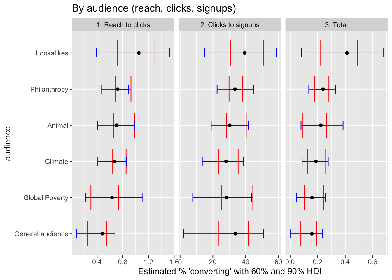
We ran two Bayesian Logit models. 20 Results come from a two-stage process: 1. some people who see the ad click on it. 2. Some of those who click on the ad leave their email (asking for a Giving Guide). We model clicks as a share of unique impressions (‘reach’) and results as a share of clicks, allowing each to vary by video theme and by audience. (Later: by text and by demographics.) The product of these shares (probabilities) yields ‘results as a share of impressions’, the main outcome of interest.
Below, we plot the point means (aka ‘coefficients’) and ‘highest density intervals’ (HDI) of our posterior beliefs for these. These models consider the audience and video themes at the same time, the imbalance between audiences and themes should probably not be a major biasing factor.
Caveats:
The specific coefficients for the second stage (‘clicks to results’) should be taken lightly; as the audiences may be selected very differently ‘conditional on click’; e.g., audiences that are ‘easy to click’ may by ‘harder to convert to a result’.
The results presented below do not control for ‘which text treatment’ nor for ‘which campaign’. (We can do the latter next, but we can only do the former with the other version of the data, which is then missing some detail on who saw which video)
The usual ‘divergent delivery’ issue
Note
Important note: the ‘pooled’ graphs (for individual audiences and videos) in this section may not be correctly weighted across subcategories. We need to reexamine this.
Code
aud_plots <- function(df) {
  df %>%
       filter(audience!="Retargeting")  %>%
    group_by(level, audience) %>% #, starts
    sum_mean_hdi %>%
    mutate(audience = reorder(as.factor(audience), `mean`)) %>%
    ggplot() +
  geom_errorbarh(aes(xmin = lower_n, xmax = upper_n, y = audience), height = .7, color = "red") +
  geom_errorbarh(aes(xmin = lower_w, xmax = upper_w, y = audience),  height=.25, color = "blue") +
  geom_point(
    aes(x=`mean`,
    y = audience))
    }

(
reach_to_clicks_aud_plot <-  full_post  %>%
    aud_plots() +
  labs(title = "By audience (reach, clicks, signups)",
       x = "Estimated % 'converting' with 60% and 90% HDI")  +
      facet_grid(~level, scales = "free")
)
Code
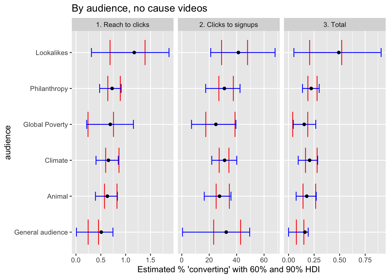
(
reach_to_clicks_aud_plot_no_cause <-  full_post  %>%
    filter(!str_det(theme, "Animal|Climate|Poverty"))  %>%
        aud_plots() +
 labs(title = "By audience, no cause videos",
       x = "Estimated % 'converting' with 60% and 90% HDI")  +
      facet_grid(~level, scales = "free")
)
Code
(
reach_to_clicks_aud_plot_cause <-  full_post  %>%
    filter(str_det(theme, "Animal|Climate|Poverty"))  %>%
        aud_plots() +
 labs(title = "By audience, Cause videos only",
       x = "Estimated % 'converting' with 60% and 90% HDI")  +
      facet_grid(~level, scales = "free")
)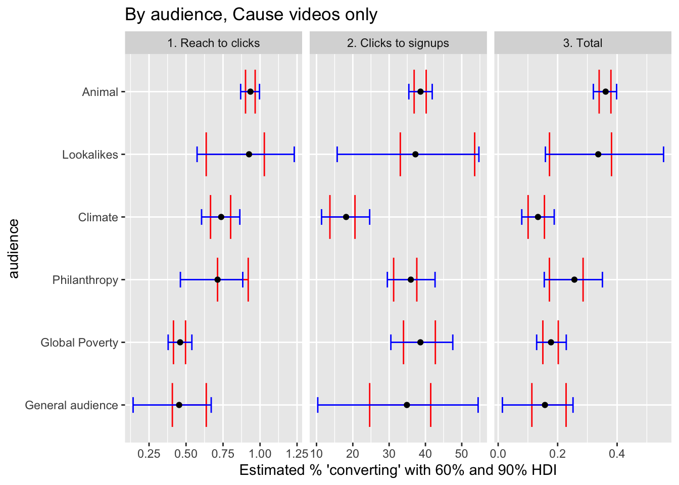
For the ‘cause videos only’ we see 21 that the philanthropy audience, across all causes, seems to perform at least as well as the climate and ‘global poverty’ audiences (when the latter are presented videos for the causes they are said to care about). However, the animal audiences seems to perform substantially better.
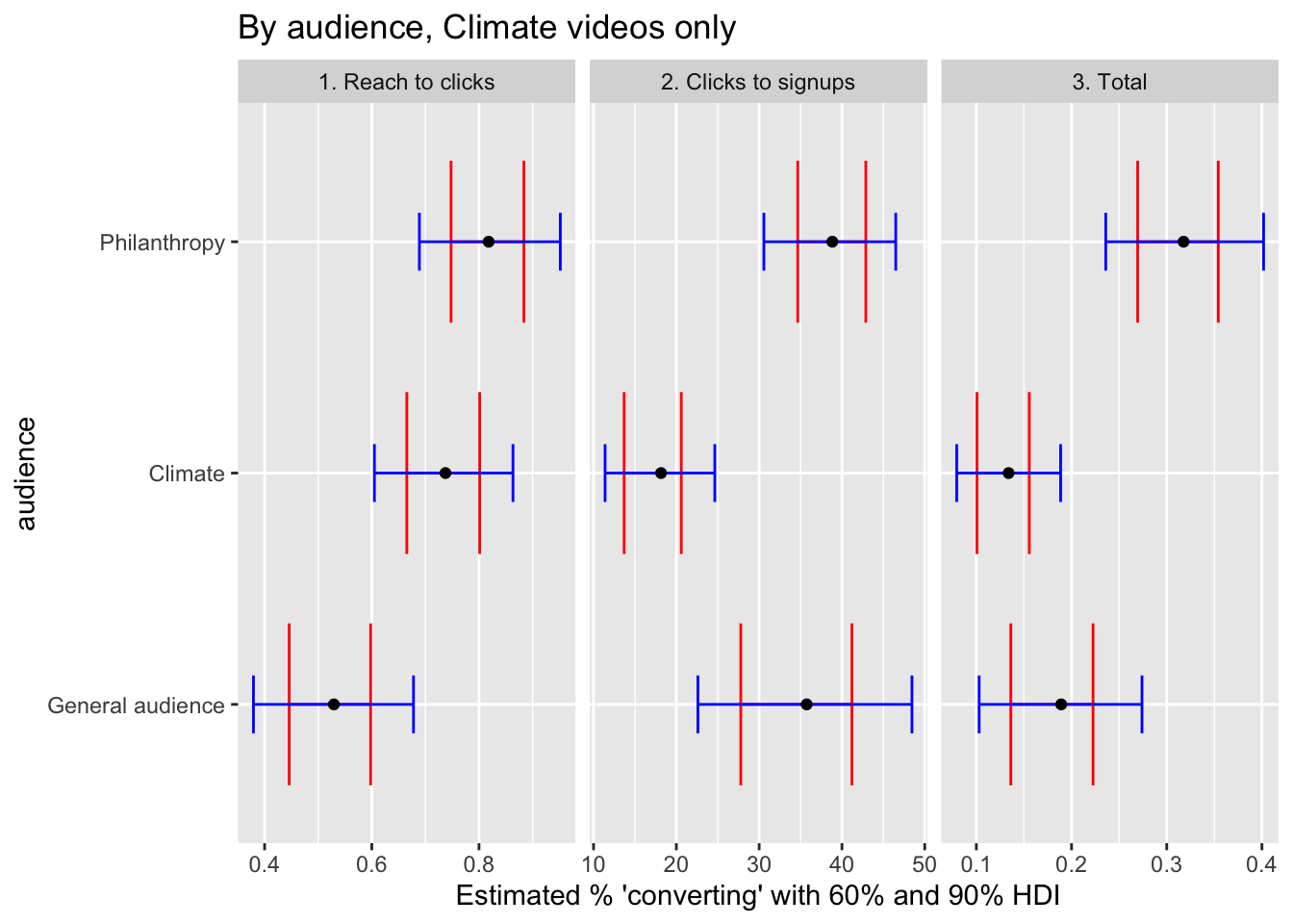
For example, focusing on climate-cause videos (and removing ‘lookalikes’) below, we see that the philanthropy audience performs substantially better than the climate audience.
Code
(
reach_to_clicks_aud_plot_climate <-  full_post  %>%
    filter(str_det(theme, "Climate"))  %>%
    filter(audience!="Lookalikes") %>%
        aud_plots() +
 labs(title = "By audience, Climate videos only",
       x = "Estimated % 'converting' with 60% and 90% HDI")  +
      facet_grid(~level, scales = "free")
)
Results by Video
Code
vid_plots <- function(df) {
df %>%
group_by(level, theme) %>% #, starts
sum_mean_hdi %>%
mutate(theme = reorder(as.factor(theme), `mean`)) %>%
ggplot() +
geom_errorbarh(aes(xmin = lower_n, xmax = upper_n, y = theme), height = .7, color = "red") +
geom_errorbarh(aes(xmin = lower_w, xmax = upper_w, y = theme), height=.25, color = "blue") +
geom_point(
aes(x=`mean`,
y = theme))
}
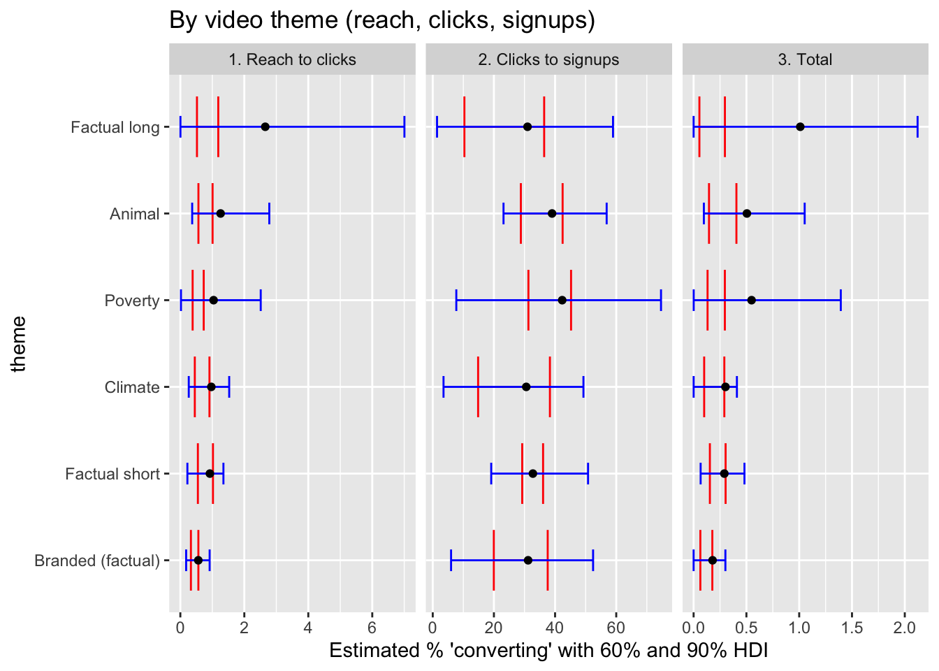
(
reach_to_clicks_vid_plot <- full_post %>%
vid_plots() +
labs(title = "By video theme (reach, clicks, signups)",
x = "Estimated % 'converting' with 60% and 90% HDI") +
facet_grid(~level, scales = "free")
)
Code
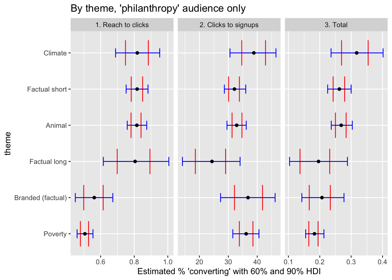
(
reach_to_clicks_vid_plot_phil <-  full_post  %>%
            filter(audience == "Philanthropy")  %>%
    vid_plots() +
  labs(title = "By theme, 'philanthropy' audience only",
       x = "Estimated % 'converting' with 60% and 90% HDI")  +
      facet_grid(~level, scales = "free")
)
Code
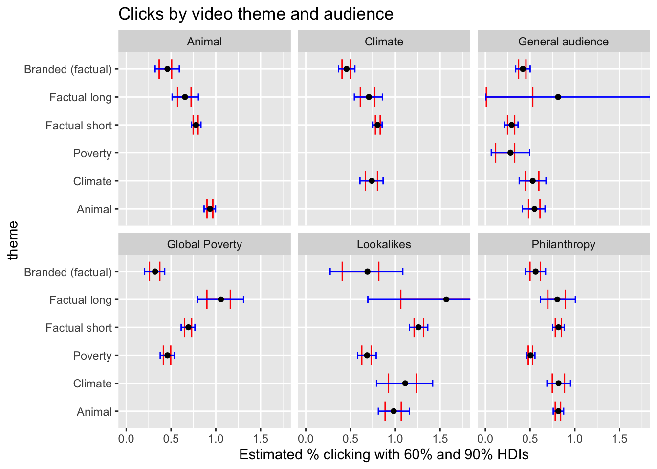
(
reach_to_clicks_plot <-  full_post  %>%
      filter(grepl("1", level)) %>%
    group_by(theme, audience) %>% #, starts
    sum_mean_hdi %>%
      mutate(theme = reorder(as.factor(theme), `mean`)) %>%
      filter(audience!="Retargeting")  %>%
    ggplot() +
  geom_errorbarh(aes(xmin = lower_n, xmax = upper_n, y = theme), height = .7, color = "red") +
  geom_errorbarh(aes(xmin = lower_w, xmax = upper_w, y = theme),  height=.25, color = "blue") +
  geom_point(aes(x = mean, y = theme)) +
  coord_cartesian(xlim=c(0, 1.75)) +
  facet_wrap(~audience, scales = "fixed") +
  labs(title = "Clicks by video theme and audience",
       x = "Estimated % clicking with 60% and 90% HDIs") +
  facet_wrap(~audience, scales = "fixed")
)
Code
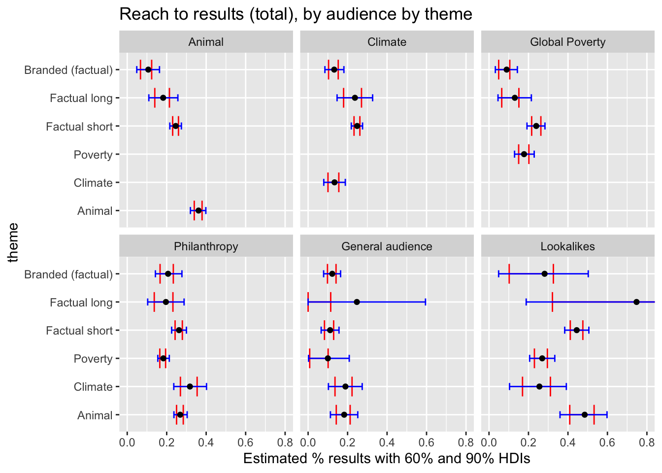
(
reach_to_results_plot <- full_post %>%
filter(grepl("3", level)) %>%
group_by(theme, audience) %>% #, startslevel,
sum_mean_hdi %>%
mutate(theme = reorder(as.factor(theme), `mean`)) %>%
filter(audience!="Retargeting") %>%
ggplot() +
geom_errorbarh(aes(xmin = lower_n, xmax = upper_n, y = theme), height = .7, color = "red") +
geom_errorbarh(aes(xmin = lower_w, xmax = upper_w, y = theme), height=.25, color = "blue") + geom_point(aes(x = mean, y = theme)) +
facet_wrap(~audience, scales = "fixed") +
coord_cartesian(xlim=c(0, 0.8)) +
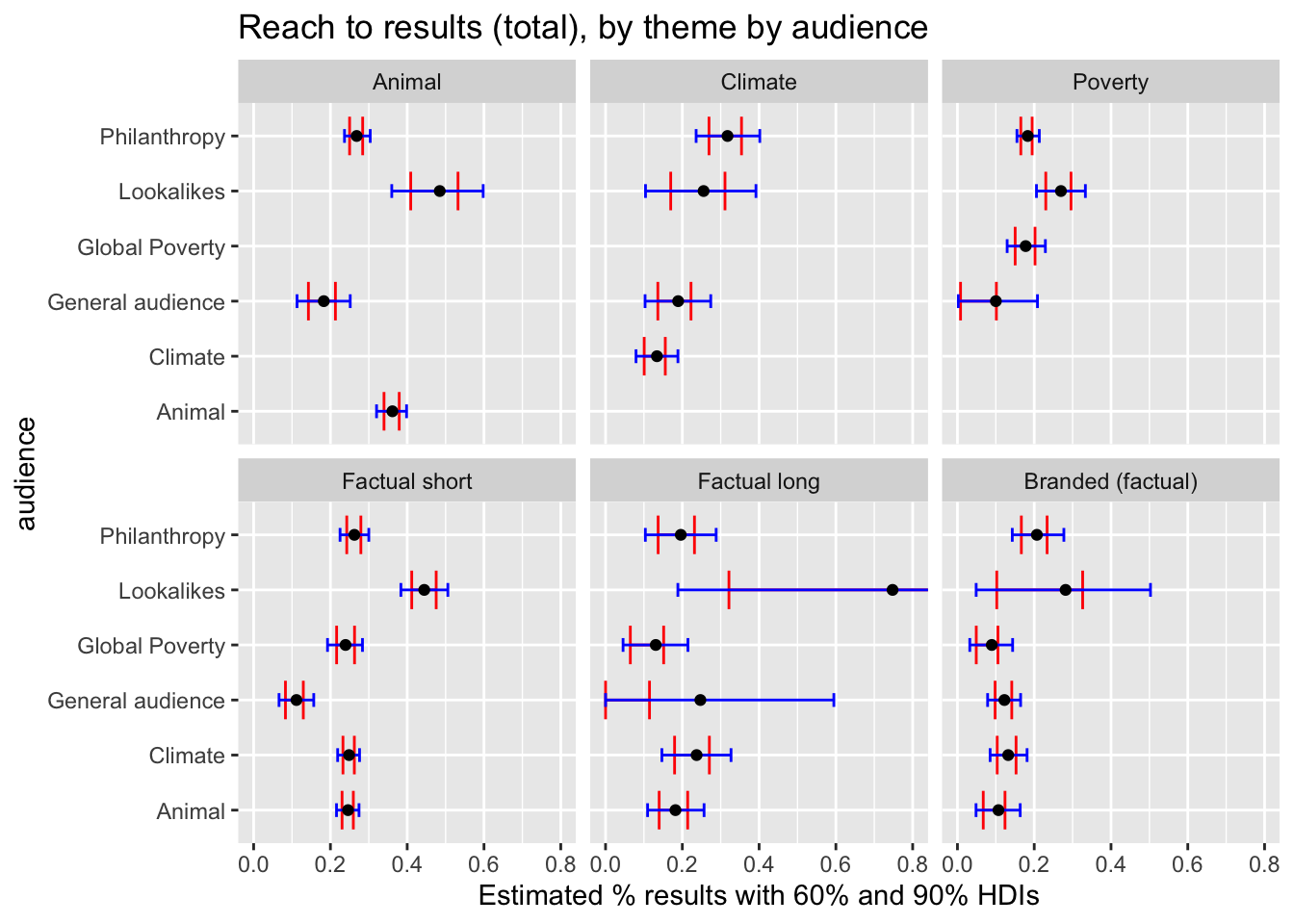
labs(title = "Reach to results (total), by audience by theme",
x = "Estimated % results with 60% and 90% HDIs") +
facet_wrap(~factor(audience, levels=audience_levels), scales = "fixed")
)
Code
(
reach_to_results_plot_flip <-  full_post %>%
      filter(grepl("3", level)) %>%
      group_by(audience, theme) %>% #, startslevel,
      sum_mean_hdi %>%
        mutate(audience = reorder(as.factor(audience), `mean`)) %>%
      filter(audience!="Retargeting")  %>%
    ggplot() +
  geom_errorbarh(aes(xmin = lower_n, xmax = upper_n, y = audience), height = .7, color = "red") +
  geom_errorbarh(aes(xmin = lower_w, xmax = upper_w, y = audience),  height=.25, color = "blue") +  geom_point(aes(x = mean, y = audience)) +
  facet_wrap(~audience, scales = "fixed") +
    coord_cartesian(xlim=c(0, 0.8)) +
  labs(title = "Reach to results (total), by theme by audience",
       x = "Estimated % results with 60% and 90% HDIs") +
  facet_wrap(~theme, scales = "fixed")
)
Results by text
Code
reach_to_results_sum_text_only <-  full_post_text_only %>%
      filter(grepl("3", level)) %>%
      group_by(text_treat) %>% #, startslevel, conte
      sum_mean_hdi( CI_choice_n=0.90, CI_choice_w = 0.99) %>%
  mutate(text_treat = reorder(as.factor(text_treat), `mean`))

reach_to_results_sum_text_only  %>%
  DT::datatable(caption = "Texts: mean performance by text, 0% and 99% HDI bounds", filter="top",  rownames= FALSE) %>%
  formatRound(1:length(reach_to_results_sum_text_only), digits=3)
Code
(
reach_to_results_sum_text_only_plot <-
reach_to_results_sum_text_only %>%
    ggplot() +
  geom_errorbarh(aes(xmin = lower_n, xmax = upper_n, y = text_treat), height = .7, color = "red") +
  geom_errorbarh(aes(xmin = lower_w, xmax = upper_w, y = text_treat),  height=.25, color = "blue") +  geom_point(aes(x = mean, y = text_treat)) +
    coord_cartesian(xlim=c(0.13, .45)) +
  labs(title = "Reach to results (total), by text",
       x = "Estimated % results with 90% and 99% HDIs")
)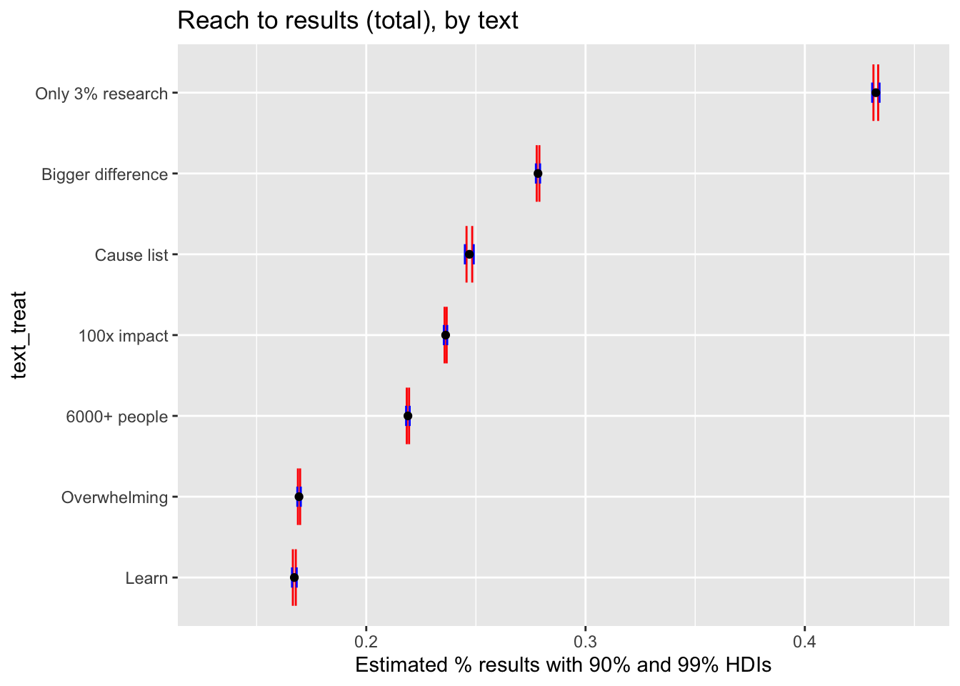
Code
reach_to_results_sum_text <-  full_post_text %>%
      filter(grepl("3", level)) %>%
      group_by(text_treat, audience) %>% #, startslevel,
      sum_mean_hdi %>%
  mutate(text_treat = reorder(as.factor(text_treat), `mean`)) %>%
      filter(audience!="Retargeting")

reach_to_results_sum_text  %>%
  DT::datatable(caption = "Texts:  mean performance by audience, 60 and 90% HDI bounds", filter="top",  rownames= FALSE) %>%
    formatRound(1:length(reach_to_results_sum_text_only), digits=3)
Code
(
reach_to_results_sum_text_plot <-
reach_to_results_sum_text %>%
    ggplot() +
  geom_errorbarh(aes(xmin = lower_n, xmax = upper_n, y = text_treat), height = .7, color = "red") +
  geom_errorbarh(aes(xmin = lower_w, xmax = upper_w, y = text_treat),  height=.25, color = "blue") +  geom_point(aes(x = mean, y = text_treat)) +
  facet_wrap(~audience, scales = "fixed") +
    coord_cartesian(xlim=c(0, .6)) +
  labs(title = "Reach to results (total), by audience by text",
       x = "Estimated % results with 60% and 90% HDIs") +
  facet_wrap(~factor(audience, levels=audience_levels), scales = "fixed")
)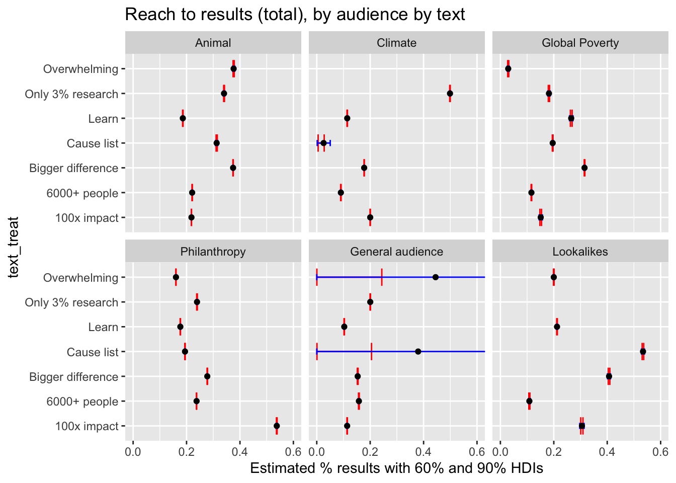
Code
(
reach_to_results_plot_flip <-  full_post_text %>%
      filter(grepl("3", level)) %>%
      group_by(audience, text_treat) %>% #, startslevel,
      sum_mean_hdi %>%
        mutate(audience = reorder(as.factor(audience), `mean`)) %>%
      filter(audience!="Retargeting")  %>%
    ggplot() +
  geom_errorbarh(aes(xmin = lower_n, xmax = upper_n, y = audience), height = .7, color = "red") +
  geom_errorbarh(aes(xmin = lower_w, xmax = upper_w, y = audience),  height=.25, color = "blue") +  geom_point(aes(x = mean, y = audience)) +
  facet_wrap(~audience, scales = "fixed") +
    coord_cartesian(xlim=c(0, 1)) +
  labs(title = "Reach to results (total), by text by audience",
       x = "Estimated % results with 60% and 90% HDIs") +
  facet_wrap(~text_treat, scales = "fixed")
)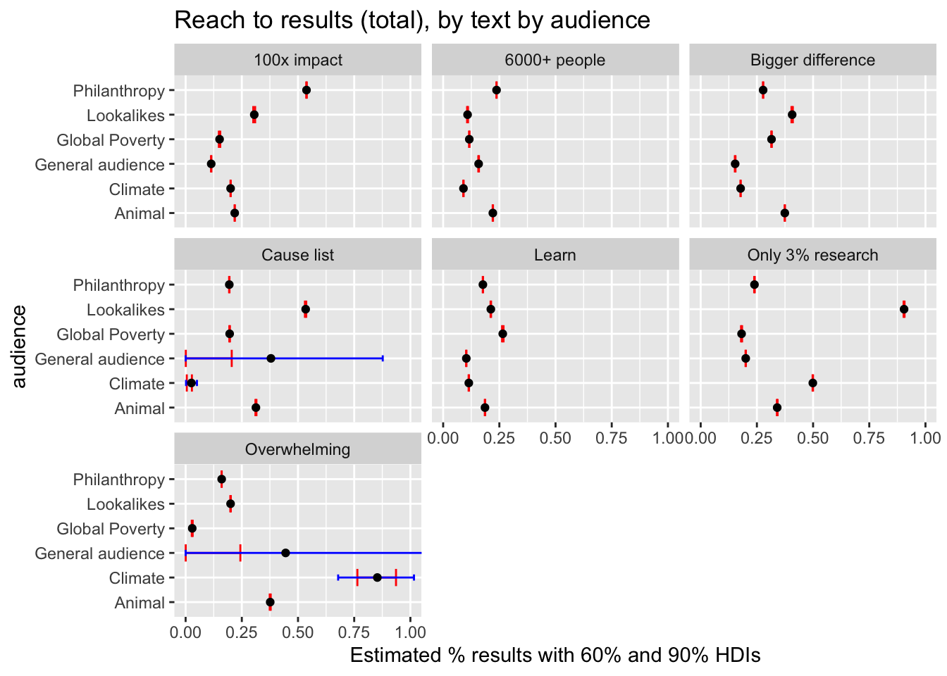
Outcomes by cost
Note: We don’t report on the ‘text’ treatment in this section (for now), because the cost per unique impression was very similar across these texts.
Code
# Joining spending and conversion ####

cost_tibble <-
  left_join(tib_combined_post,
    rename(gg_video_breakdowns_col, theme=video_theme)) %>%
  mutate(
    reach_per_dollar = reach / spend,
    sign_per_dollar = reach_per_dollar * probability,
    #NOTE this uses the simulated distribution of probabilities, not just averages!
    sign_per_100d = 100*sign_per_dollar,
    cost_per_signup = 1/sign_per_dollar
    ) %>%
  filter(is.na(spend) == FALSE)

cost_summary <- cost_tibble %>%
  group_by(theme, audience) %>%
  sum_mean_hdi(var= sign_per_100d, scaleme=1)

#dim(filter(cost_summary, check > 2))[1] ... where HDI is not continuous, I guess... this doesn't happen here atm
Code
(
  sign_per_100d_plot_vid_by_aud <- cost_tibble %>%
      filter(audience!="Retargeting")  %>%
ggplot() +
  scale_x_continuous(limits = c(0, 20)) +
  ggridges::geom_density_ridges(
    aes(
      x = sign_per_100d,
      y = theme
      )
    ) +
  geom_point(data = cost_summary %>% filter(audience!="Retargeting"),
    aes(x = mean, y = theme)) +
  labs(title = "Signups per $100: Comparing videos by audience",
    x = "Density plots, means") +
  facet_wrap(~factor(audience, levels = audience_levels), scales = "free_x"  )
)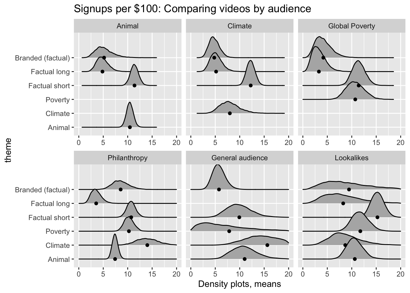
Code
#
# ggplot(filter(cost_tibble, upper_eti < 100)) +
#   geom_errorbarh(aes(xmin = lower_eti, xmax = upper_eti, y = audience)) +
#   geom_point(aes(x = mean, y = audience)) +
#   labs(title = "Cost per signup ($)",
#     x = "Estimated cost per signup (USD) with 95% ETI") +
#   facet_wrap(~theme, scales = "free_x")
Above we consider the cost effectiveness of each video by audience.
‘Factual short’: 23 This video seems to perform as good or better than any other video for each of the cause audiences as well as for the Lookalike audience (but see cav eat). It performs nearly as good as other videos for the other audiences.
Climate video: This seems to have performed best for the Philanthropy and General audiences, although the distribution is diffuse. Surprisingly, it does not perform best for the climate audience.
Brand Video, Factual Long: These seemed to have performed worst or near-worst for most audiences. ‘Factual long’ seems to have clearly performed worse than ‘Factual short’ version. (But see caveat below.)
Caveat/todo – Video/campaign date imbalance
There is substantial imbalance in dates the administration of treatments in the pooled data. E.g., the ‘Factual short’ video was the only one shown for the 2021-12-08 trial, which may confound the above result. The Brand Video was only shown in a single trial, where it was the only video shown. The ‘Factual long’ video was dropped in later trials (possibly after poor performance in an explicit A/B test). Again, confounds are certainly possible. We may want to either remove trials from dates that only ran a single trial (at a first pass), or include start date/campaign into our modeling.
Code
(
  sign_per_100d_plot_aud_by_vid <- cost_tibble %>%
      filter(audience!="Retargeting" & audience!="General audience")  %>%
ggplot() +
  scale_x_continuous(limits = c(0, 20)) +
  ggridges::geom_density_ridges(
    aes(
      x = sign_per_100d,
      y = audience
      )
    ) +
  geom_point(data = cost_summary %>% filter(audience!="Retargeting" & audience!="General audience"),
    aes(x = mean, y = audience)) +
  labs(title = "Signups per $100: Comparing audiences for each video",
    x = "Density plots, means") +
  facet_wrap(~theme, scales = "free_x")
)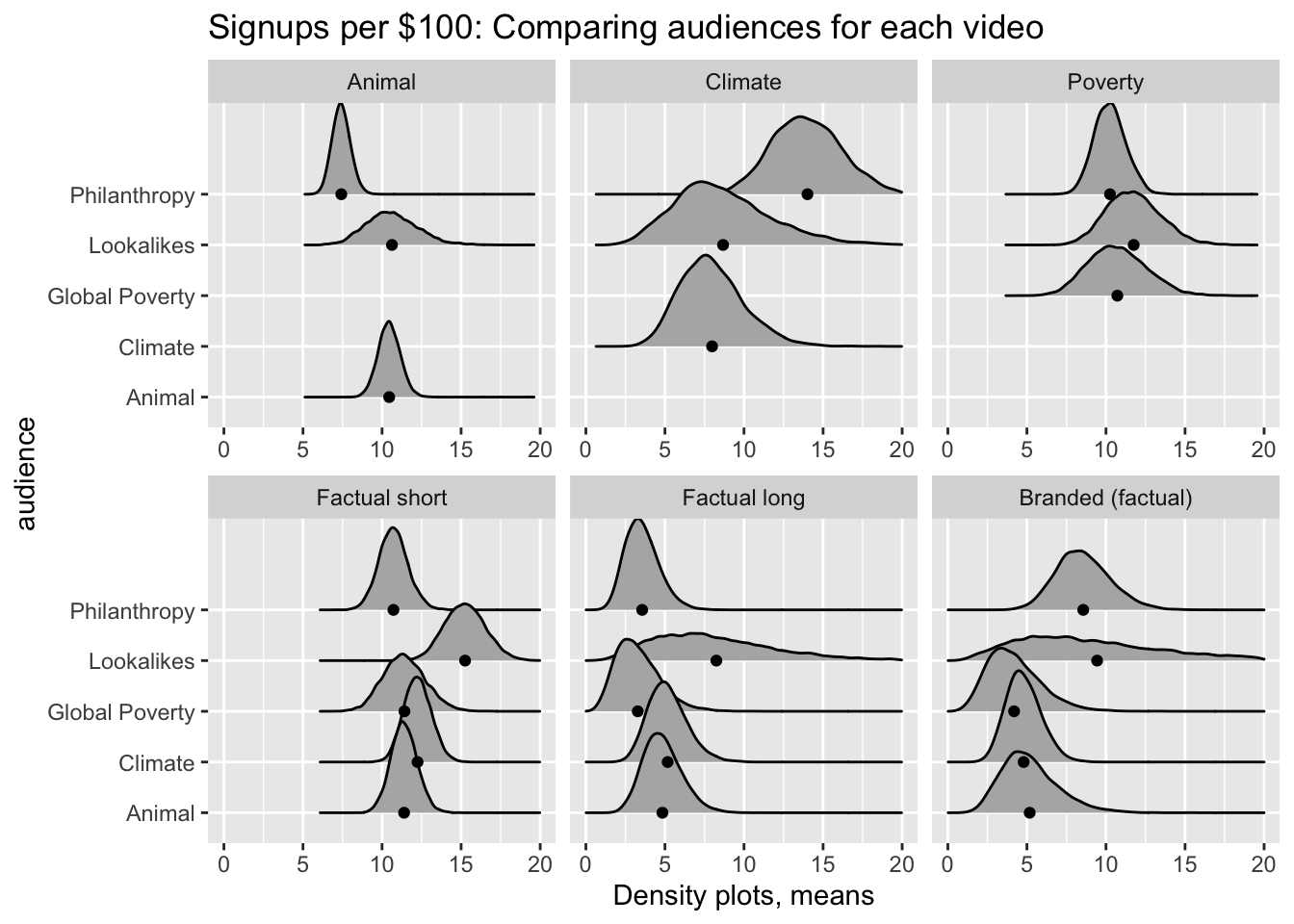
Flipping the previous plot, we compare the cost-effectiveness of each audience for each video.24, 25
The Lookalike audiences are relatively cost-effective for most videos, although the Philanthropy audience seems to do better per dollar for the Climate video.
The cause audiences are relatively cost-effective for their ‘own’ videos, but not overwhelmingly so. They seemed particularly cost-ineffective for the Brand video.
See ‘which videos’ below for a list and brief descrription of these audiences.↩︎
As well as the third dimension of ‘different targeted audiences’.↩︎
We see ‘no individuals over 45’ in the data for all experiments starting after mid-December↩︎
We use the latter going forward as it subsumes the former; the former is just kept as a check.↩︎
However, for the Brand Video campaign these are further broken up; I am not sure how.↩︎
In particular, it seems that for the
Giving Guide 2021 – PPCo CreativestheEmotional + Factual (Animated)draws from a different set of ads for (e.g.)Global Poverty + Lookalikes (18-39)versusPhilanthropy + Lookalikes (18-39). I assume it draws from all causes for non-cause-linked audiences, but for the cause-linked audiences it draws only from the cause-of-interest, as well as the general ‘factual’ videos.↩︎Unfortunately, for these groups, we cannot extract the data on which cause-specific video they saw in combination with certain other categories, like ‘which text’ or demographics. This breaks up our analysis a bit.↩︎
This also may lead FB to particularly combine certain message presentations more with certain video presentations. However we cannot check this in our current setup: it is confounded with ‘audience profile’ (at least in the data we can observe).↩︎
We suspect Facebook’s algorithm uses some version of Thompson sampling to optimize along the explore/exploit frontier.↩︎
But we essentially excluded the 13-17 age group, completely excluding it in later.↩︎
Todo: present or link at least something here about the likely dispersion/CI’s for these. We should have a sense of ‘how strong’ these differences are. A minor challenge: we run the models and simulations later, so this would make this Quarto less of a ‘transparent pipeline’.↩︎
But recall we cannot distinguish which cause message they were shown for this slice of the data.↩︎
Here we could have included the cause audiences and it would have been somewhat comparable, but we leave them out for simplicity↩︎
But on a results per impression, the lookalikes seem do substantially better, and the cause-led treatments do better among the Philanthropy audience.↩︎
We can also use the data that includes information on the video all audiences saw here, because we don’t need to filter on message.↩︎
Developers note: all of this description is hard-coded.↩︎
In some cases these had few observations, which we believe was because Facebook’s algorithm largely ‘gave up on these’ videos for this audience because of very poor performance.↩︎
this text is ‘hard-coded’ on 4 Aug 2022 … if data changes we need to change the text↩︎
Tech note: the video names in the previous sentence are soft-coded, i.e., inline code; see the previous chunk where we identify the
top_vid_philandbot_vid_phil.↩︎TODO: tables summarizing these models themselvees↩︎
todo: doublecheck after final estimates↩︎
Todo: fix weighting↩︎
Hard-coded, may need recoding after fixes↩︎
Again hard-coding here…↩︎
Note that the audience-imbalance caveat still applies. We removed the ‘General Audience’ here, as this was only used for the final trial, and this seems particularly non-comparable.↩︎