6 Control strategies and prediction, Machine Learning (Statistical Learning) approaches
6.1 See also “notes on Data Science for Business”
‘Identification’ of causal effects with a control strategy not credible
Essentially a ‘control strategy’ is “control for all or most of the reasonable determinants of the independent variable so as to make the remaining unobservable component very small, minimizing the potential for bias in the coefficient of interest.” All of the controls must still be exogenous, otherwise this itself can lead to a bias. There is some discussion of how to validate this approach; see, e.g., (osterUnobservableSelectionCoefficient2019?). ## Machine Learning (statistical learning): Lasso, Ridge, and more
Machine learning seeks to fit models to data in order to learn patterns and thus make predictions about the future. This learning is split into categories:
Supervised learning: Here our data consists of labelled examples. This means that we have data on the outcome variable of interest. Linear regression is a form of supervised learning algorithm as the data used will contain values for \(Y\) and is thus labeled.
Unsupervised learning: In this type of learning data has no label. Clustering algorithms are examples of unsupervised learning, where the model seeks to group objects into collections with other similar observations.
Semi-supervised learning: This method is used in order to account for the high cost of labeling data. Where a data set may have labels for some observations and not for others we use semi-supervised learning.
Reinforcement learning: Reinforcement learning works by assigning rewards (or errors) to actions taken by an algorithm. Typically this reward will be an estimate of how much reward is received at the end of a round. This method is popular in artificial intelligence programs, such as the AlphaGo algorithm by DeepMind.
6.1.1 Limitations to inference from learning approaches
From a discussion on the EA forum about predicting donation choices
… the ML approaches Greg is suggesting here are all about prediction, not about drawing meaningful inferences.For prediction it’s good to start with the largest amount of features (variables) you can find (as long as they are truly ex-ante) and then do a fancy dance of cross-validation and regularisation, before you do your final ‘validation’ of the model on set-aside data.But that doesn’t easily give you the ability to make strong inferential statements (causal or not), about things like ‘age is likely to be strongly associated with satisfaction measures in the true population.’ Why not? If I understand correctly:The model you end up with, which does a great job at predicting your outcome
… may have dropped
ageentirely or “regularized it” in a way that does not yield an unbiased or consistent estimator of the actual impact ofageon your outcome. Remember, the goal here was prediction, not making inferences about the relationship between of any particular variable or sets of variables …… may include too many variables that are highly correlated with the
agevariable, thus making the age coefficient very imprecise… may include variables that are actually ‘part of the age effect you cared about, because they are things that go naturally with age, such as mental agility’
Finally, the standard ‘statistical inference’ (how you can quantify your uncertainty) does not work for these learning models (although there are new techniques being developed)
6.1.2 Tree models
This section was mainly written by Oska Fentem.
Decision trees are a type of supervised machine learning algorithm. While they are very simple and intuitive to understand, they form the basis for a variety of more complex models. Here we will discuss the model in the context of a classification problem; however they can also be used for continuous outcome (‘regression’) settings.
Decision trees are a type of supervised machine learning algorithm. “Recursive binarry splitting” is used; the algorithm repeatedly splits the data into subsets and subsets of these subsets, finally making a prediction based on the dominant group in each subset. A decision tree consists of:
- Root node: this is the first node in the tree.
- Interior nodes: these are the nodes on which the data is split.
- Leaf nodes: these contain the final classifications made by the model.
In splitting a data set by it’s features (variables) the decision tree algorithm seeks to split using the most informative features first. In order to calculate which features are the most informative we can calculate information gain or Gini impurity.
6.1.2.1 Information Gain
Information gain is used to measure the feature which provides the largest increase in information about the classification of our outcome variable. This metric is based on the notion of entropy, a measure of set impurity as well as the remaining information.
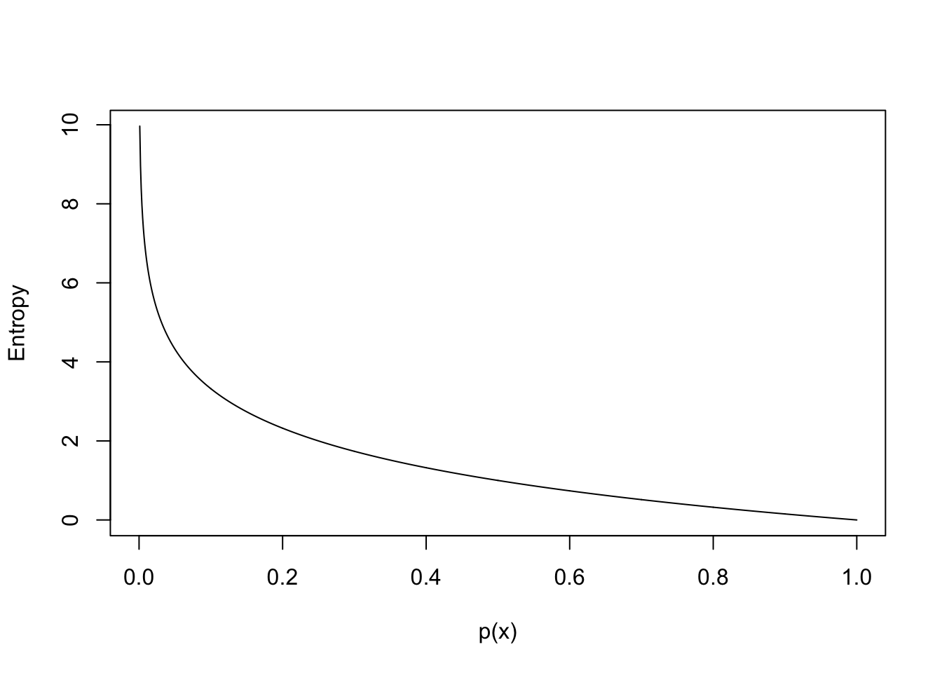
Entropy: For \(X = x_1,…, x_n\) occurring with probability \(P(x_1),…, P(x_n)\) entropy is defined as: \[\text{Entropy} = -\sum_{i=1}^n P(x_i)\log_2 P(x_i)\] Entropy is high when there is more uncertainty around the result if we were to guess a member of the set at random. An example of a set with high entropy would be a pack of playing cards. Each card in the set has a low probability of being picked. This means that we would be very uncertain about the outcome of picking a card at random. By graphing the function \(- P(x_i) \log_2 P(x_i)\) we see that as the probability of an each outcome decreases the total entropy increases:
Using the entropy function we are able to compute information gain with the following three equations:
\[ \begin{aligned}&\operatorname{rem}(d, \mathcal{D})=\sum_{I \in \text {levels}(d)} \underbrace{\frac{\left|\mathcal{D}_{d=I}\right|}{|\mathcal{D}|}}_{\text {weighting }} \times \underbrace{H\left(t, \mathcal{D}_{d=I}\right)}_{\text {entropy of partition} \space \mathcal{D}_{d=I}}\\&I G(d, \mathcal{D})=H(t, \mathcal{D})-\operatorname{rem}(d, \mathcal{D})\end{aligned} \]
Source: (Kelleher, Mac Namee, and D’Arcy 2015)
6.1.2.2 Ensemble learning
Decision trees provide an easy and intuitive way to represent a complex relationships between \(X\) and \(Y\). While these models have very low bias they have high variance. This means that changes in the training data may cause large changes in the predictions made by the model.
Random forests are a form of ensemble learning. This method works by combining multiple weaker classifiers into one strong one. By doing this we average the predictions made across all the decision trees, which can often result in better performance than a single tree. In a random forest we fit multiple decision tree models on random bootstrap sub-samples of our data, limiting ourselves, in each forest, to a randomly-restricted subset of variables (features). The algorithm works as follows:
For \(b=1\) to \(B\):
Draw a bootstrap sample \(Z^*\) of size \(N\) from our training data
- Select a subset of \(m\) variables by random out of a total of \(p\) variables
Use this sample to fit a tree, \(T_b\):
Pick the best variable to split the data on out of \(m\)
Split the node
Steps i-ii are repeated until the minimum node size is reached.
Output ensemble
Note that this procedure is similar to bagging. However, by using a random set of \(m\) variables to consider for splitting our nodes the random forest algorithm achieves lower correlation between the individual trees. Standard bagging instead makes use of all \(p\) variables when deciding on tree splits, which could result in trees that are correlated. If we have a collection of identically distributed trees then the expectation of all these models is equal to the expectation of any one of them. If one tree is more likely to make a wrong prediction this is averaged out by the lack of correlation between this and the other models.
As forests contain a collection of smaller trees the prediction process is slightly different than for individual trees. Consider that each tree gives a prediction \(\hat{C}_b(X)\). Our random forest prediction is thus: \[\hat{C}_{rf}^B = \text{Majority vote} \{ \hat{C}_n)x_i \}^B_1\]
Source: (friedmanElementsStatisticalLearning2001?)
6.2 Notes Hastie: Statistical Learning with Sparsity
6.2.1 Introduction
One form of simplicity is sparsity, the central theme of this book. Loosely speaking, a sparse statistical model is one in which only a relatively small number of parameters (or predictors) play an important role.
“the \(\ell_1\) norm is special” (abs value). Other norms yield nonconvex problems, hard to minimize.
“bet on sparsity” principle: Use a procedure that does well in sparse problems, since no procedure does well in dense problems.
- Examples from gene mapping
6.2.1.1 Book roadmap
Chapter 2 … lasso for linear regression, and a simple coordinate descent algorithm for its computation.
Chapter 3 application of \(\ell_1\) [lasso-type] penalties to generalized linear models such as multinomial and survival models, as well as support vector machines. [?]
Chapter 4: Generalized penalties such as the elastic net and group lasso are discussed in Chapter 4.
Chapter 5: numerical methods for optimization (skip for now]
Chapter 6: statistical inference for fitted (lasso) models, including the bootstrap, Bayesian methods and more recent stuff
Chapter 7: Sparse matrix decomposition [?] (Skip?)
Ch 8: sparse multivariate analysis of that (Skip?)
Ch 9: Graphical models and their selection (Skip?)
Ch 10: compressed sensing (Skip?)
Ch 11: a survey of theoretical results for the lasso (Skip?)
6.2.2 Ch2: Lasso for linear models
- N samples (?N observations), want to approx the response variable using a linear combination of the predoctors
OLS minimizes squared-error loss but
- Prediction accuracy
OLS unbiased but ‘often has large variance’
prediction accuracy can be improved by shrinking coefficients (even to zero)
- yielding biased but perhaps better predictive estimators
- Interpretation: too many predictors hard to interpret
- DR: I do not care about this for fitting background noise in experiments
6.2.2.1 2.2 The Lasso Estimator
Lasso bounds the sum of the abs values of coefficients, an “$_1” constraint.
Lasso is OLS subject to
\(\sum_{j=1..p}{\abs(\beta_j)}\leq t\)
“compactly” \(||\beta||_1\leq t\)
with notation for the “\(\ell_1\) norm”
Bound \(t\) acts as a ‘budget,’ must be specified by an ‘external procedure’ such as cross-validation
typically we must standardize the predictors $** so that each column is centered with unit variance … as well as the outcome variables (?) … can ignore intercept
- DR: Not clear here whether standardisation is necessary for the procedure to be valid or just convenient for explaining and deriving its properties.
Aside: Can re-write Lasso minimization st constraint as a Lagrangian. \(\lambda\) plays the same role as \(t\) in the constraint. Thus we can speak of the solution to the Lagrangian minimisation problem \(\hat{\beta)_{\lambda}\) which also solves the bound problem with \(t=||\hat_{\lambda}||_1\).
Aside: We often remove the \(1/2n\) term at the beginning of the minimization problem. Same minimization, minimizing sum of squared deviations rather than something like an average of this.
Express (Karush-Kuhn-Tucker) optimisation conditions for this …
Example from Thomas (1990) on crime data
Typically … lasso is most useful for much larger problems, including “wide” data for which \(p>>N\)
Fig 2.1: Lasso vs ridge regression; coefficients of each for a set of considered variables plotted against their respective norms (as shares of maximal bound on coefficient sum measure, i.e., ols, for each)
Note ridge regression penalises squared sums of betas
- Fig 2.2., in \(\beta_1,\beta_2\) space illustrates the difference well: contour lines of Resid SS elipses, ‘budget constraint’ for each (disc vs diamond)
(Note: lasso bound was chosen via cross-validation)
- No analytical statistical inference after lasso (some being developed?), bootstrap is common
lasso sets two of the five coefficients to zero, and tends to shrink the coefficients of the others toward zero relative to the full least-squares estimate.
DR: analytically and intuitively, I do not yet understand why lasso should shrink coefficients but not all the way to zero.
- The penalty is linear in the coefficient size, so I would think the solution would be bang-bang, either drop a coeficient or leave it unchanged. But it is not.
- Adding an increment to a \(\hat{\beta}\) when it is below the OLS estimate should have a linear effect on the RSS (according to my memory and according to Sebastian).
- But that would mean that shrinking one parameter always yields a better benefit to cost ratio. Thus I should shrink each parameter to zero before beginning to shrink any others. This cannot be right!
I looked up this derivative wrt the beta vector (one needs to set this to 0 to get the ols estimates
\(\frac{d RSS}{d \beta}=-2X^{T}(y-X\beta}\)
or
\(−\frac{d e'e}{d b}=2X′y+2X′Xb\)
The answer to this question: while the impact of changing each coefficient on SSR is in fact constant (a constant own-derivative), there is also an impact of changing one coefficient on the other derivatives. As one coefficient shrinks to zero the marginal impact of the other coefficients on the SSR may (will?) increase.
- At the same time, we need that the effect of increasing it from zero need not be infinite, so it might not outweigh the linear penalty, thus some coefficients might be set to zeroRelaxed lasso
the least-squares fit on the subset of the three predictors tends to expand the lasso estimates away from zero. The nonzero estimates from the lasso tend to be biased toward zero, so the debiasing in the right panel can often improve the prediction error of the model. This two-stage process is also known as the relaxed lasso (Meinshausen 2007).
DR: When is this likely to help/hurt relative to pure lasso?
Stackexchange discussion Contrasts a ‘relaxed-lasso’ from a ‘lars-ols’
Aside: which seems better for Control variable selection for prediction/reducing noise to enable better inference of treatment effects?
Ridge? better than Lasso here? We do not care about interpreting the predictors here… so if we allow \(\beta\)’s to be shrunk towards zero for each coefficient maybe that should yield better prediction than making them exactly zero?
On the other hand if we know the true model is ‘parsimonious’ (as in the genes problem) it might boost efficiency to allow inference about coefficients that should be exactly zero (edited)
6.2.2.2 2.3 Cross-Validation and Inference
- Generalization ability
accuracy for predicting independent test data from the same population
… find the value of t that does best
**Cross-validation procedure*
- randomly divide … dataset into K groups.
“Typical choices … might be 5 or 10, and sometimes N.”
One ‘test,’ remaining K-1 ‘training’
Apply lasso to training data for a range of t values,
- use each fitted model to predict the responses in the test set, recording mean-squared prediction errors for each value of t.
Repeat the previous step K times
- each time, one of the K groups is the test data, remaining K − 1 are training data.
- yields K different estimates of the prediction error over a range of t values.
Average K estimates of prediction error for each value of t \(\rightarrow\) cross-validation error curve.
Fig 2.3 plots an example with K=10 splits for cross validation
- … of the estimated MS prediction error vs the relative bound \(\tilde{t}\)(summed absolute value of Lasso betas divided by summed abs value of OLS betas).
- Also draw dotted line at the 1-std-error rule choice of \(\tilde{t\)}
- Number of nonzero coefficients plotted at top
6.2.2.3 2.4 Computation of the Lasso solution
DR: I think I will skip this for now
least angle/LARS is mentioned at the bottom as a ‘homotopy method’ which “produce the entire path of solutions in a sequential fashion, starting at zero”
6.2.2.4 2.5 Degrees of freedom
…
Jumping to
6.2.2.5 2.10 Some perspective
Good properties of the Lasso (\(\ell_1\) penalty)
Natural interpretation (enforce sparsity and simplicity)
Statistical efficiency … if the underlying true signal is sparse (but if it is not sparse “no method can do well relative to the Bayes error”)
Computational efficiency, as \(\ell_1\) penalties are convex
6.2.3 Chapter 3: Generalized linear models
6.2.4 Chapter 4: Generalizations of the Lasso penalty
lasso does not handle highly correlated variables very well; the coefficient paths tend to be erratic and can sometimes show wild behavior.
The elastic net makes a compromise between the ridge and the lasso penalties (Zou and Hastie 2005)1] is a parameter that can be varied.
For an individual coefficient the penalty is \(\frac{1}{2} (1-\alpha)\beta_j^2 + \alpha|\beta_j|\)
(a convex combo of the lasso and ridge penalties)
multiplied by a ‘regularization weight’ \(\lambda>0\) which plays the same role (I think) as in lasso
- elastic net is also strictly convex
6.3 Notes: Mullainathan
The fundamental insight behind these breakthroughs is as much statistical as computational. Machine intelligence became possible once researchers stopped approaching intelligence tasks procedurally and began tackling them empirically. Face recognition algorithms, for example, do not consist of hard-wired rules to scan for certain pixel combinations, based on human understanding of what constitutes a face. Instead, these algorithms use a large dataset of photos labeled as having a face or not to estimate a function f (x) that predicts the presence y of a face from pixels x
(p2) > supervised- machine learning, the focus of this article) revolves around the problem of prediction: produce predictions of y from x
…
manages to fit complex and very flexible functional forms to the data without simply overfitting; it finds functions that work well out-of-sample
danger in using these tools is taking an algorithm built for [predicting \(y\)-] and presuming their [parameters \(\beta\)] - have the properties we typically associate with estimation output
One category of such applications appears when using new kinds of data for traditional questions; for example, in measuring economic activity using satellite images or in classifying industries using corporate 10-K filings. Making sense of complex data such as images and text often involves a prediction pre-processing step
This middle category is most relevant for me
In another category of applications, the key object of interest is actually a parameter … but the inference procedures (often implicitly) contain a prediction task. For example, the first stage of a linear instrumental variables regression is effectively prediction. The same is true when estimating heterogeneous treatment effects, testing for effects on multiple outcomes in experiments, and flexibly controlling for observed confounders
A final category is in direct policy applications. Deciding which teacher to hire implicitly involves a prediction task (what added value will a given teacher have?), one that is intimately tied to the causal question of the value of an additional teacher.
(p3)
A useful (interactive?) example:
We consider 10,000 randomly selected owner-occupied units from the 2011 metropolitan sample of the American Housing Survey. In addition to the values of each unit, we also include 150 variables that contain information about the unit and its location, such as the number of rooms, the base area, and the census region within the United States. To compare different prediction techniques, we evaluate how well each approach predicts (log) unit value on a separate hold-out set of 41,808 units from the same sample. All details on the sample and our empirical exercise can be found in an online appendix available with this paper at http://e-jep.org
In-sample performance may overstate performance; this is especially true for certain machine learning algorithms like random forests that have a strong tendency to overfit. Second, on out-of-sample performance, machine learning algorithms such as random forests can do significantly better than ordinary least squares, even at moderate sample sizes and with a limited number of covariates
(p4)
algorithms are fitted on the same, randomly drawn training sample of 10,000 units and evaluated on the 41,808 remaining held-out units.
Simply including all pairwise interactions would be infeasible as it produces more regressors than data points (especially considering that some variables are categorical
Machine learning searches for these interactions automatically
(p5)
Shallow Regression Tree Predicting House Values
not sure what’s going on here. is this the random forest thing?
The prediction function takes the form of a tree that splits in two at every node. At each node of the tree, the value of a single variable (say, number of bathrooms) determines whether the left (less than two bathrooms) or the right (two or more) child node is considered next. When a terminal node-a leaf—is reached, a prediction is returned. An
So how does machine learning manage to do out-of-sample prediction? The first part of the solution is regularization. In the tree case, instead of choosing the -best" overall tree, we could choose the best tree among those of a certain depth.
(p5) Tree depth is an example of a regularizer. It measures the complexity of a function. As we regularize less, we do a better job at approximating the in-sample variation, but for the same reason, the wedge between in-sample and out-of-sample
(p6) how do we choose the level of regularization (-tune the algorithm")? This is the second key insight: empirical tuning.
(p6) -tuning within the training sample In empirical tuning, we create an out-of-sample experiment inside the original sample. We fit on one part of the data and ask which level of regularization leads to the best performance on the other part of the data.4 We can increase the efficiency of this procedure through cross-validation: we randomly partition the sample into equally sized subsamples (-folds"). The estimation process then involves successively holding out one of the folds for evaluation while fitting the prediction function for a range of regularization parameters on all remaining folds. Finally, we pick the parameter with the best estimated average performance.5 The
(p6) -! This procedure works because prediction quality is observable: both predictions y- and outcomes y are observed. Contrast this with parameter estimation, where typically we must rely on assumptions about the data-generating process to ensure consistency
(p7) Some Machine Learning Algorithms Function class - (and its parametrization) Regularizer R( f ) Global/parametric predictors Linear -′x (and generalizations) Subset selection|
(p7) -very useful table Some Machine Learning Algorithms Function class - (and its parametrization) Regularizer R( f ) Global/parametric predictors Linear -′x (and generalizations) Subset selection||β|
(p7) Random forest (linear combination of trees
(p7) -kernel in an ml framework! Kernel regression
(p6) -but can we make inferences about the structure? hypothesis testing? Regularization combines with the observability of prediction quality to allow us to fit flexible functional forms and still find generalizable structure.
(p7) Picking the prediction function then involves two steps: The first step is, conditional on a level of complexity, to pick the best in-sample loss-minimizing function.8 The second step is to estimate the optimal level of complexity using empirical tuning (as we saw in cross-validating the depth of the tree).
(p8) -but they forgot to mention that others are shrunk linear regression in which only a small number of predictors from all possible variables are chosen to have nonzero values: the absolute-value regularizer encourages a coefficient vector where many are exactly zero.
(p4) -why no ridge or elastic net? LASSO
(p8) -ensembles usually win contests While it may be unsurprising that such ensembles perform well on average- after all, they can cover a wider array of functional forms-it may be more surprising that they come on top in virtually every prediction competition
(p8) -neural nets broadly explained neural nets are popular prediction algorithms for image recognition tasks. For one standard implementation in binary prediction, the underlying function class is that of nested logistic regressions: The final prediction is a logistic transformation of a linear combination of variables (-neurons") that are themselves such logistic transformations, creating a layered hierarchy of logit regressions. The complexity of these functions is controlled by the number of layers, the number of neurons per layer, and their connectivity (that is, how many variables from one level enter each logistic regression on the next)
(p9) These choices about how to represent the features will interact with the regularizer and function class: A linear model can reproduce the log base area per room from log base area and log room number easily, while a regression tree would require many splits to do so.
(p9) In a traditional estimator, replacing one set of variables by a set of transformed variables from which it could be reconstructed would not change the predictions, because the set of functions being chosen from has not changed. But with regularization, including these variables can improve predictions because-at any given level of regularization-the set of functions might change
(p9) -!! Economic theory and content expertise play a crucial role in guiding where the algorithm looks for structure first. This is the sense in which -simply throw it all in- is an unreasonable way to understand or run these machine learning algorithms
(p9) -I need hear of using adjusted r square for this Should out-ofsample performance be estimated using some known correction for overfitting (such as an adjusted R2 when it is available) or using cross-validation
(p9) -big unknowns available finite-sample guidance on its implementation-such as heuristics for the number of folds (usually five to ten) or the -one standard-error rule" for tuning the LASSO (Hastie, Tibshirani, and Friedman 2009)-has a more ad-hoc flavor
(p9) firewall principle: none of the data involved in fitting the prediction function-which includes crossvalidation to tune the algorithm—is used to evaluate the prediction function that is produced
(p10) -how? First, econometrics can guide design choices, such as the number of folds or the function class
(p10) with the fitted function. Why not also use it to learn something about the -underlying model
(p10) -!! the lack of standard errors on the coefficients. Even when machine-learning predictors produce familiar output like linear functions, forming these standard errors can be more complicated than seems at first glance as they would have to account for the model selection itself. In fact, Leeb and P-tscher (2006, 2008) develop conditions under which it is impossible to obtain (uniformly) consistent estimates of the distribution of model parameters after data-driven selection
(p11) -lasso chosen variables are unstable because of multicollinearity. a problem for making inferences from estimated coefficients the variables are correlated with each other (say the number of rooms of a house and its square-footage), then such variables are substitutes in predicting house prices. Similar predictions can be produced using very different variables. Which variables are actually chosen depends on the specific finite sample
(p11) this creates an Achilles- heel: more functions mean a greater chance that two functions with very different
(p12) coefficients can produce similar prediction quality
(p12) In econometric terms, while the lack of standard errors illustrates the limitations to making inference after model selection, the challenge here is (uniform) model selection consistency itself
(p12) -is this equally a problem for non sparsity based procedures like ridge? First, it encourages the choice of less complex, but wrong models. Even if the best model uses interactions of number of bathrooms with number of rooms, regularization may lead to a choice of a simpler (but worse) model that uses only number of fireplaces. Second, it can bring with it a cousin of omitted variable bias, where we are typically concerned with correlations between observed variables and unobserved ones. Here, when regularization excludes some variables, even a correlation between observed variables and other observed (but excluded) ones can create bias in the estimated coefficients
(p12) Some econometric results also show the converse: when there is structure, it will be recovered at least asymptotically (for example, for prediction consistency of LASSO-type estimators in an approximately sparse linear framework, see Belloni, Chernozhukov, and Hansen 2011).
(p12) -unrealistic for micro economic applications Zhao and Yu (2006) who establish asymptotic model-selection consistency for the LASSO. Besides assuming that the true model is -sparse“—only a few variables are relevant-they also require the”irrepresentable condition" between observables: loosely put, none of the irrelevant covariates can be even moderately related to the set of relevant ones. In practice, these assumptions are strong.
(p13) Machine learning can deal with unconventional data that is too high-dimensional for standard estimation methods, including image and language information that we conventionally had not even thought of as data we can work with, let alone include in a regression
(p13) satellite data
(p13) they provide us with a large x vector of image-based data; these images are then matched (in what we hope is a representative sample) to yield data which form the y variable. This translation of satellite images to yield measures is a prediction problem
(p13) particularly relevant where reliable data on economic outcomes are missing, such as in tracking and targeting poverty in developing countries (Blumenstock 2016
(p13) cell-phone data to measure wealth
(p13) Google Street View to measure block-level income in New York City and Boston
(p13) online posts can be made meaningful by labeling them with machine learning
(p14) extract similarity of firms from their 10-K business description texts, generating new time-varying industry classifications for these firms
(p14) and imputing even in traditional datasets. In this vein, Feigenbaum (2015a, b) applies machine-learning classifiers to match individuals in historical records
(p13) -the first prediction applications New Data
(p14) Prediction in the Service of Estimation
(p14) linear instrumental variables understood as a two-stage procedure
(p14) The first stage is typically handled as an estimation step. But this is effectively a prediction task: only the predictions x- enter the second stage; the coefficients in the first stage are merely a means to these fitted values. Understood this way, the finite-sample biases in instrumental variables are a consequence of overfitting
(p14) -ll overfitting. Overfitting means that the in-sample fitted values x- pick up not only the signal -′z, but also the noise δ. As a consequence, xˆ is biased towards x, and the second-stage instrumental variable estimate - - is thus biased towards the ordinary least squares estimate of y on x. Since overfit will be larger when sample size is low, the number of instruments is high, or the instruments are weak, we can see why biases arise in these cases
(p14) same techniques applied here result in split-sample instrumental variables (Angrist and Krueger 1995) and -jackknife" instrumental variables (Angrist, Imbens, and Krueger 1999)
(p15) -worth referencing In particular, a set of papers has already introduced regularization into the first stage in a high-dimensional setting, including the LASSO (Belloni, Chen, Chernozhukov, and Hansen 2012) and ridge regression (Carrasco 2012; Hansen and Kozbur 2014). More recent extensions include nonlinear functional forms, all the way to neural nets (Hartford, Leyton-Brown, and Taddy 2016
(p15) Practically, even when there appears to be only a few instruments, the problem is effectively high-dimensional because there are many degrees of freedom in how instruments are actually constructed
(p15) -a note of caution It allows us to let the data explicitly pick effective specifications, and thus allows us to recover more of the variation and construct stronger instruments, provided that predictions are constructed and used in a way that preserves the exclusion restriction
(p15) -this seems similar to my idea of regularising on a subset Chernozhukov, Chetverikov, Demirer, Duflo, Hansen, and Newey (2016) take care of high-dimensional controls in treatment effect estimation by solving two simultaneous prediction problems, one in the outcome and one in the treatment equation
(p15) the problem of verifying balance between treatment and control groups (such as when there is attrition
(p15) -! Or consider the seemingly different problem of testing for effects on many outcomes. Both can be viewed as prediction problems (Ludwig, Mullainathan, and Spiess 2017). If treatment assignment can be predicted better than chance from pretreatment covariates, this is a sign of imbalance. If treatment assignment can be predicted from a set of outcomes, the treatment must have had an effect
(p15) prediction task of mapping unit-level attributes to individual effect estimates
(p15) Athey and Imbens (2016) use sample-splitting to obtain valid (conditional) inference on
(p16) treatment effects that are estimated using decision trees,
(p16) -look into the implication for treatment assignment with heterogeneity heterogenous treatment effects can be used to assign treatments; Misra and Dub- (2016) illustrate this on the problem of price targeting, applying Bayesian regularized methods to a large-scale experiment where prices were randomly assigned
(p16) -caveat Suppose the algorithm chooses a tree that splits on education but not on age. Conditional on this tree, the estimated coefficients are consistent. But that does not imply that treatment effects do not also vary by age, as education may well covary with age; on other draws of the data, in fact, the same procedure could have chosen a tree that split on age instead
(p16) Prediction in Policy
(p16) -no .. can we predict who will gain most from admission? but even if we can what can we report? Prediction in Policy