7 Data please!

7.1 Why do we use data?
Just like Johnny-five and his cousin the Robot cash register, Economists need ‘input’ from the real world to improve our understanding.
Descriptive
To measure and understand our object of study: the economy (including individuals, households, firms, and governments)
Levels of variables, patterns (e.g., Life cycle consumption),
observed relationships between variables (differences by group, correlations, linear relationships, etc.)
For its own sake
To use in executing policy (e.g., the Consumer Price Index)
To generate hypotheses and “calibrate” our models
We can have statistical tests of “descriptive” hypothesis.
E.g., testing
H0: Incomes of men and women are the same ceteris paribus vs. HA: Women with the same characteristics as men earn less on average.
Note: this is not testing a causal relationship;
a difference doesn’t necessarily imply a particular explanation (e.g., sex discrimination).
Causal: To make statistical inferences (and statistical predictions) about effects
(sometimes called “causal effects” but I find that redundant).
To measure and test hypotheses about the causal relationship between important factors and outcomes.
7.2 What data do you need to answer your question?
Look for data that is…
RELEVANT to your topic
the relevant population, years, fields;
relevant outcome variable(s), “independent variable(s)” of interest, control variables)
USEFUL for answering your question: E.g., it contains a useful “instrumental variable”, a long enough time series, or repeated observations on individuals to allow ‘fixed effects’ controls.
Reliable, accessible, understandable
Consider previous work: What data have PREVIOUS AUTHORS used to answer this or related questions?
7.3 Some types of data
- Survey and collected data: self-reports, interviewers, physical measures and visual checks
- Administrative data (e.g., tax records)
- Transactions/interactions
- Scanner data
- Web data (e.g., Ebay, Amazon)
- Price data
- Public financial data and company reports
- Official government data (public releases and announcements, e.g., budget data)
- Data from lab experiments
- Data from field experiments
Consider the differences between:
Micro-data (individual/transaction level) vs. Macro-data (aggregated to firm, region, country-year level etc)
Panel vs cross-section vs time-series data
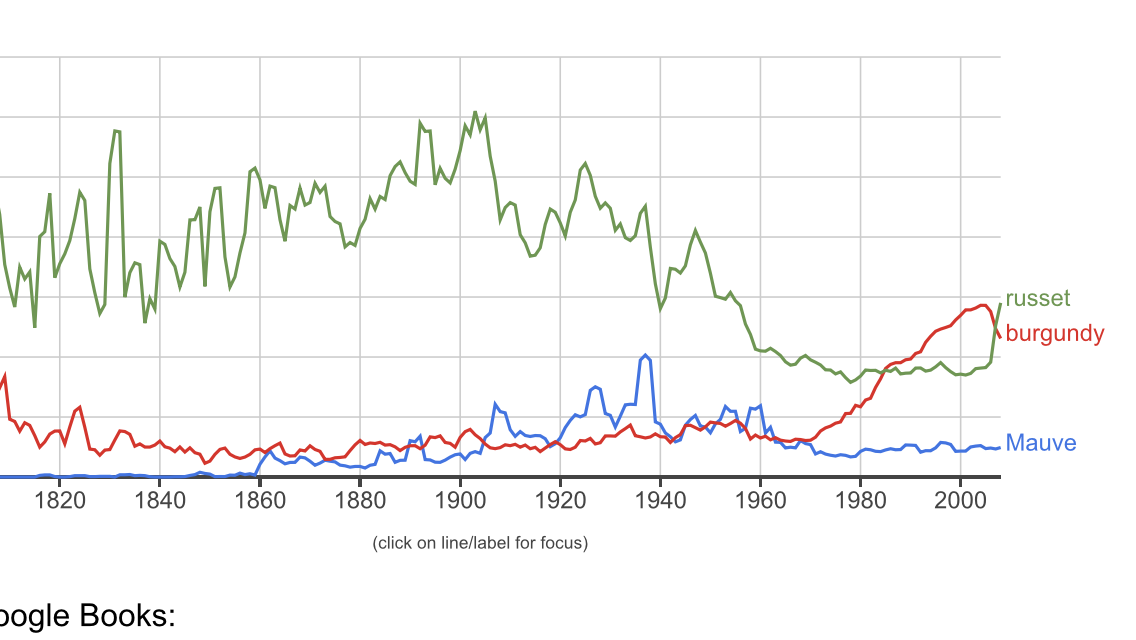
Figure 7.1: A graph based on a new type of data
Some examples of datasets used by Undergraduate students
Unfold…
Workplace Employee Relations Survey: Private Sector Panel, 1998-2004 data, from the UK Data Archive.
Data on cigarette consumption from the US Centers of Disease Control (CDC) from 1986 to 2011, for 50 states \(\rightarrow\) 1300 observations.
The 1958 National Child Development Survey, a longitudinal study tracking a group of individuals born in a single week in 1958.
Data on UK cities’ population, employment, geography, extracted from various ONS tables.
“The ICCSR UK Environmental & Financial Dataset, is a large panel data set on a a sample of firms, giving a set of ratings on “community and environmental responsibility”; merged to a set of financial variables on these firms, collected from Datastream
Exchange rates between the US dollar, the British pound, Australian dollar, Canadian dollar and Swiss franc, for the period 1975-2010, from the OECD Main Economic Indicators database.
The World Bank Development Indicator database (2013); 210 countries over a 20-year period from 1991-2010
65 banks over 8 years from BankScope (profitability measures, etc)
7.4 Getting and using data
Finding data
Update: A particularly promising resource: Google dataset search
In searching for data, note that the American Economics Association has a very comprehensive list of links: http://www.aeaweb.org/RFE/toc.php?show=complete for the UK in specific, see http://www.statistics.gov.uk/default.asp
For macro and micro data, see http://www.esds.ac.uk/
For large scale data, see also the UK Data Service database.
Some other sources of data, and links to aggregations on my webpage here.
My database of resources:
Some of these (and lists of lists) are also listed in this Airtable also mentioned below… this is filtered ‘data search/archive’; remove this filter to see more.
Also, to comment on this you can get full ‘commenter’ access link
Also note that data from published papers are typically expected to be made publicly accessible (for replication and checking purposes). If you cannot find it on the journal or the author’s website (or linked therein), you can email the corresponding author to ask for it.
Don’t wait too long to begin collecting your data and producing simple graphs and summary statistics, to get a sense of your data.
Empirical work is difficult and you may not be able to get the “best” data. This is OK. Remember, at the undergraduate/MSc level, we generally want you to show your competencies in these assignments; we expect the analysis will have limitations.
7.4.1 Downloading the data, raw formats
The most common format to download the data in is ‘csv’ for ‘comma-separated values.’ This can be read into Stata, R, and nearly any program.
The first row usually gives the variable names, which you can change later in your program.
Commas separate each variable (aka ‘feature’ aka ‘column’).
Each observation (aka ‘unit’ aka ‘row’) is separated by a line break.
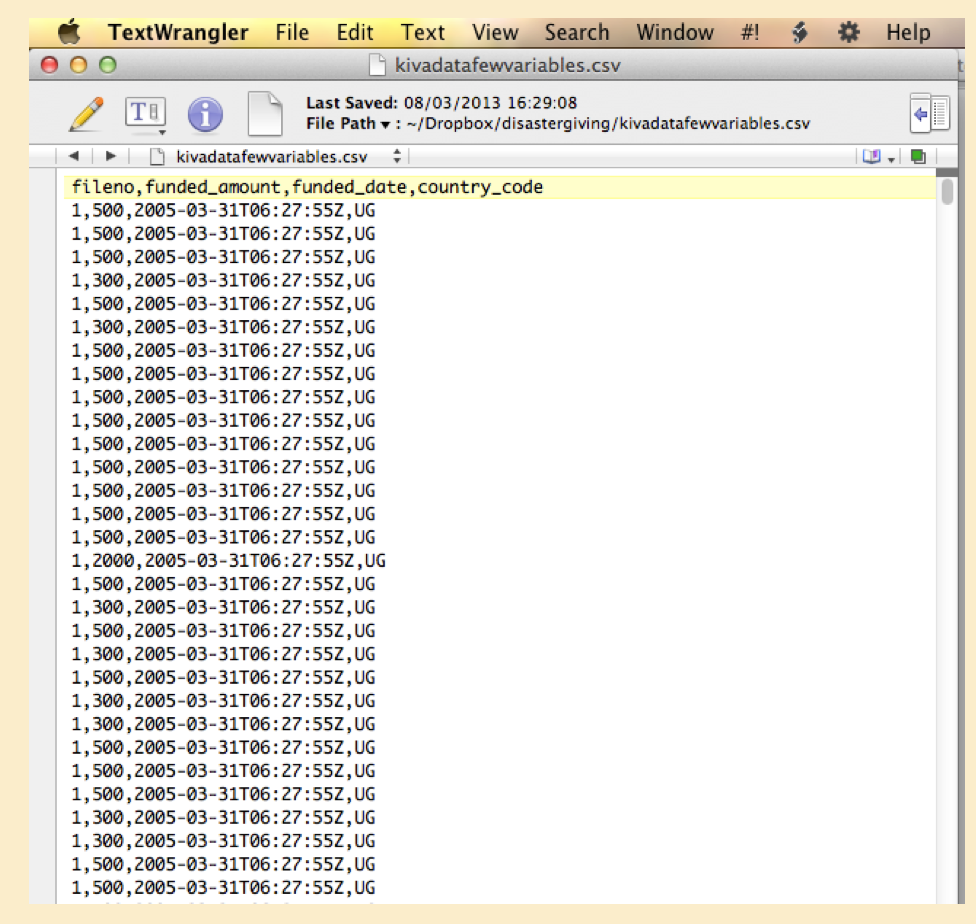
Figure 7.2: Raw data viewed in a text editor
(See ‘Text editors’ below.)
What is a ‘plain (flat) text file’?
A “flat text file” is different from (e.g.) a Word document (.docx)
The Word document is a fancy complicated file or collection of files that has all sorts of sneaky hidden stuff and can only be viewed by MS Word or other similar applications.
A ‘text file’ is simply just ASCII or UTF text, some basic elements for your computer.
It’s filename often has the extension .txt but it doesn’t need to. It can have any extension, such as .md to indicate that it’s markdown, .tex for Latex, .R for R code, .Rmd for R-markdown, .do for a Stata do file, etc.
In writing computer programs and content we basically always use ‘flat text files.’ How do you create/edit these? You need to use a ‘text editor’.
(See ‘Text editors’ below.)
Inputting the data (into Stata, R, etc)
These programs have several ‘input’ commands you can use (e.g., insheet in Stata, read_csv in R) for “getting the data in” (as an object that can be referred to and analyzed).
You could use the ‘drop-down’ menu or some other visual tool perhaps, to input it, but this is not best practice.3 Find the right input command and make this part of your code. (See ‘Doing coding…’.)
7.5 Understanding your data
Present simple statistics and graphics on your data before doing more involved analyses.
7.6 What does data look like (brief)
Inputting raw data (in R)
Author’s note: I hope to soon update this to display these types of data directly through R, especially using the built-in datasets.
‘Data’ is simply an organised expression of information. You may be most familiar with seeing it in spreadsheets like MS Excel.
Let’s start from “raw data” as mentioned above. This often refers to a “flat text file”… just a file that contains a bunch of characters and numbers and line breaks, essentially. This may be something that you:
- downloaded or accessed directly from a data archive (or database or API or other repository),
Both R and Stata have tools that allow you to directly input data from a web resource without even downloading it. One advantage of this is that it can be automatically updated as the data updates on the external site.
stripped from a web page with a ‘cut and paste’ or using the tools of ‘web scraping’ etc.,
collected yourself through a survey or experiment (ideally using a tool that didn’t require you to hand-code everything),
or input by hand in some way; but avoid please hand-input because:
- useful data sets can be large and more data generally yields greater statistical power and
- you can make errors in hand-input, and you may need to input more later, and this does not make the process replicable.
You may be used to seeing such files stored as something.txt but actually they can be stored with any extension.
There are standard “raw” formats that data is stored in, such as ‘comma separated values’ or ‘csv’, usually a file called something.csv.
Each “row” of a csv file will contain one “unit” or “observation”, e.g.:
14677, 'Bazooka Joe', 'Male', 25, 50000
The first row may contain the column headers or “variable names” (or, in data science “feature” names):
'id', 'name', 'sex', 'age', 'annual_income_nominal'
Between each row is some form of ‘carriage return’ … to indicate a new line.
So, for example, the raw csv file sweet_people.csv may look like:
id, name, sex, age, annual_income_nominal
14677, 'Bazooka Joe', 'male', 25, 50000
14678, 'Mary Jane', 'female', 30, 65000
…. with many more possible rows (or columns of course.
In the above view, you do not see any symbol indicating a carriage return between lines; you can view this in a text editor by choosing to ‘see hidden characters’ or something similar.
In R, if I can help R locate the file sweet_people.csv on my hard drive or on a web-accessible location, I can view the raw file or input it as a ‘dataframe’ or ‘tibble’ for manipulation and analysis:
| id | name | sex | age | annual_income_nominal |
|---|---|---|---|---|
| 14677 | 'Bazooka Joe' | 'male' | 25 | 50000 |
| 14678 | 'Mary Jane' | 'female' | 30 | 65000 |
The above R code will only work if the file sweet_people.csv is stored in the subfolder sample_data within R’s current working directory.
The first line inputs the file using the read.csv command and stores it as the object sweet_ppl. The second line simply displays this object. We can see each variable (or ‘feature’) name in the first (bold) row. Below it, in
What kind of object is sweet_ppl from the point of view of the R language? We can check with the command
str(sweet_ppl):
## 'data.frame':    2 obs. of  5 variables:
##  $ id                   : int  14677 14678
##  $ name                 : chr  " 'Bazooka Joe'" " 'Mary Jane'"
##  $ sex                  : chr  " 'male'" " 'female'"
##  $ age                  : int  25 30
##  $ annual_income_nominal: int  50000 65000
I actually prefer to use the tidyverse and Magritr syntax, so I would code sweet_ppl %>% str(), after installing the appropriate packages.
I would also convert this dataframe into a ‘tibble’, a slight variation on a data frame (in the way it’s displayed).
See https://r4ds.had.co.nz/ for more on these concepts.
… We see that R refers to this as a “data frame”, which is one of the most important basic objects in R.
Note that read.csv is not the only command for inputting data, although it is probably the simplest. Both R and Stata have commands to directly input data from Excel spreadsheets (.xlsx) and many other formats.
7.6.1 Types of data, viewing and summarizing it
There are several ‘formats’ of data… considering how it is divided into observational units, time periods, and characteristics. This is discussed below.
R has a variety of built in data, mainly for practicing with and doing examples, but some of which is interesting for actual analysis. These data sets are mainly rather small, with few observations and few variables. (Stata also has a set of built in datasets.)
You can see detailed a list of all of these by typing the command data() … just the names of these are listed below.
##   [1] "ability.cov"           "airmiles"              "AirPassengers"
##   [4] "airquality"            "anscombe"              "attenu"
##   [7] "attitude"              "austres"               "beaver1"
##  [10] "beaver2"               "BJsales"               "BJsales.lead"
##  [13] "BOD"                   "cars"                  "ChickWeight"
##  [16] "chickwts"              "co2"                   "CO2"
##  [19] "crimtab"               "discoveries"           "DNase"
##  [22] "esoph"                 "euro"                  "euro.cross"
##  [25] "eurodist"              "EuStockMarkets"        "faithful"
##  [28] "fdeaths"               "Formaldehyde"          "freeny"
##  [31] "freeny.x"              "freeny.y"              "HairEyeColor"
##  [34] "Harman23.cor"          "Harman74.cor"          "Indometh"
##  [37] "infert"                "InsectSprays"          "iris"
##  [40] "iris3"                 "islands"               "JohnsonJohnson"
##  [43] "LakeHuron"             "ldeaths"               "lh"
##  [46] "LifeCycleSavings"      "Loblolly"              "longley"
##  [49] "lynx"                  "mdeaths"               "morley"
##  [52] "mtcars"                "nhtemp"                "Nile"
##  [55] "nottem"                "npk"                   "occupationalStatus"
##  [58] "Orange"                "OrchardSprays"         "PlantGrowth"
##  [61] "precip"                "presidents"            "pressure"
##  [64] "Puromycin"             "quakes"                "randu"
##  [67] "rivers"                "rock"                  "Seatbelts"
##  [70] "sleep"                 "stack.loss"            "stack.x"
##  [73] "stackloss"             "state.abb"             "state.area"
##  [76] "state.center"          "state.division"        "state.name"
##  [79] "state.region"          "state.x77"             "sunspot.month"
##  [82] "sunspot.year"          "sunspots"              "swiss"
##  [85] "Theoph"                "Titanic"               "ToothGrowth"
##  [88] "treering"              "trees"                 "UCBAdmissions"
##  [91] "UKDriverDeaths"        "UKgas"                 "USAccDeaths"
##  [94] "USArrests"             "UScitiesD"             "USJudgeRatings"
##  [97] "USPersonalExpenditure" "uspop"                 "VADeaths"
## [100] "volcano"               "warpbreaks"            "women"
## [103] "WorldPhones"           "WWWusage"
Let’s look at one of these in more detail. Type ?swiss to get a description of this data frame.
This would be considered ‘cross sectional’ data: it pertains to a set of units (each of 47 Swiss provinces) at a particular point in time (the year 1888). It is also ‘aggregated’ data, as (almost all) columns contain an average for that province, rather than an observation for a particular individual living in that province.
To view this entire data set we can just type its name, and it will show up in the console:
swiss
| Fertility | Agriculture | Examination | Education | Catholic | Infant.Mortality |
|---|---|---|---|---|---|
| 80.2 | 17 | 15 | 12 | 9.96 | 22.2 |
| 83.1 | 45.1 | 6 | 9 | 84.8 | 22.2 |
| 92.5 | 39.7 | 5 | 5 | 93.4 | 20.2 |
| 85.8 | 36.5 | 12 | 7 | 33.8 | 20.3 |
| 76.9 | 43.5 | 17 | 15 | 5.16 | 20.6 |
| 76.1 | 35.3 | 9 | 7 | 90.6 | 26.6 |
| 83.8 | 70.2 | 16 | 7 | 92.8 | 23.6 |
| 92.4 | 67.8 | 14 | 8 | 97.2 | 24.9 |
| 82.4 | 53.3 | 12 | 7 | 97.7 | 21 |
| 82.9 | 45.2 | 16 | 13 | 91.4 | 24.4 |
| 87.1 | 64.5 | 14 | 6 | 98.6 | 24.5 |
| 64.1 | 62 | 21 | 12 | 8.52 | 16.5 |
| 66.9 | 67.5 | 14 | 7 | 2.27 | 19.1 |
| 68.9 | 60.7 | 19 | 12 | 4.43 | 22.7 |
| 61.7 | 69.3 | 22 | 5 | 2.82 | 18.7 |
| 68.3 | 72.6 | 18 | 2 | 24.2 | 21.2 |
| 71.7 | 34 | 17 | 8 | 3.3 | 20 |
| 55.7 | 19.4 | 26 | 28 | 12.1 | 20.2 |
| 54.3 | 15.2 | 31 | 20 | 2.15 | 10.8 |
| 65.1 | 73 | 19 | 9 | 2.84 | 20 |
| 65.5 | 59.8 | 22 | 10 | 5.23 | 18 |
| 65 | 55.1 | 14 | 3 | 4.52 | 22.4 |
| 56.6 | 50.9 | 22 | 12 | 15.1 | 16.7 |
| 57.4 | 54.1 | 20 | 6 | 4.2 | 15.3 |
| 72.5 | 71.2 | 12 | 1 | 2.4 | 21 |
| 74.2 | 58.1 | 14 | 8 | 5.23 | 23.8 |
| 72 | 63.5 | 6 | 3 | 2.56 | 18 |
| 60.5 | 60.8 | 16 | 10 | 7.72 | 16.3 |
| 58.3 | 26.8 | 25 | 19 | 18.5 | 20.9 |
| 65.4 | 49.5 | 15 | 8 | 6.1 | 22.5 |
| 75.5 | 85.9 | 3 | 2 | 99.7 | 15.1 |
| 69.3 | 84.9 | 7 | 6 | 99.7 | 19.8 |
| 77.3 | 89.7 | 5 | 2 | 100 | 18.3 |
| 70.5 | 78.2 | 12 | 6 | 99 | 19.4 |
| 79.4 | 64.9 | 7 | 3 | 98.2 | 20.2 |
| 65 | 75.9 | 9 | 9 | 99.1 | 17.8 |
| 92.2 | 84.6 | 3 | 3 | 99.5 | 16.3 |
| 79.3 | 63.1 | 13 | 13 | 96.8 | 18.1 |
| 70.4 | 38.4 | 26 | 12 | 5.62 | 20.3 |
| 65.7 | 7.7 | 29 | 11 | 13.8 | 20.5 |
| 72.7 | 16.7 | 22 | 13 | 11.2 | 18.9 |
| 64.4 | 17.6 | 35 | 32 | 16.9 | 23 |
| 77.6 | 37.6 | 15 | 7 | 4.97 | 20 |
| 67.6 | 18.7 | 25 | 7 | 8.65 | 19.5 |
| 35 | 1.2 | 37 | 53 | 42.3 | 18 |
| 44.7 | 46.6 | 16 | 29 | 50.4 | 18.2 |
| 42.8 | 27.7 | 22 | 29 | 58.3 | 19.3 |
But there are other ways to look at this data; and for larger data sets ‘seeing all the data at once’ may be overwhelming both for you and for your computer.
Another way to see the whole data set is with the ‘View’ command, i.e., View(swiss) (or, using the pipe, swiss %>% View()). This will bring up an ‘Viewer’ interface that will look familiar to those accustomed to spreadsheets.
For large data sets it is more practical to look at or summarise only subsets of this data, selecting only certain rows and columns, or printing only summary statistics.
One way to do this is with the ‘head’ command, which displays only the ‘first part’ of this.
head(swiss)
| Fertility | Agriculture | Examination | Education | Catholic | Infant.Mortality |
|---|---|---|---|---|---|
| 80.2 | 17 | 15 | 12 | 9.96 | 22.2 |
| 83.1 | 45.1 | 6 | 9 | 84.8 | 22.2 |
| 92.5 | 39.7 | 5 | 5 | 93.4 | 20.2 |
| 85.8 | 36.5 | 12 | 7 | 33.8 | 20.3 |
| 76.9 | 43.5 | 17 | 15 | 5.16 | 20.6 |
| 76.1 | 35.3 | 9 | 7 | 90.6 | 26.6 |
There are many many other ways of viewing (or storing) parts of data, producing summary statistics, and visualising the data. It’s worth learning about these in some detail. For R, I recommend the R for data science guide.
To learn what any command or function does in R, simply type the command in the console with a “?” in front, e.g., type ?head to learn more about the head command.
7.7 Missing Data
This sub-section is a work in progress being written by Oska Fentem, an Economics student at Exeter, under the supervision of Dr. David Reinstein.
It is highly likely that when performing data analysis, you will run into the issue of missing data. Missing data can have an impact on resulting analysis and this impact will vary according to the underlying cause of the missingness. Therefore it is important to identify the cause of missing data.
We will discuss this further below; although this section is a work in progress.
Missing Data and Software
In Stata missing values are represented as a dot . and are coded as positive infinity.
It is important to be aware of this coding when using comparison operators like the ‘greater than’ \(>\) sign.
In R missing values are represented as NA. Unlike in Stata, R does not code missing values as an extremely large or small number. This means that missing values cannot be used in logical evaluations, such as NA > 1.
When data is read into R, NA values are automatically identified as being missing. However, it is very common for datasets to have missing values represented by other values such as N/A, na or even numbers such as 99. The option na.strings can be used to set the values which represent missing data when importing it into R.
R automatically excludes all cases in which any of the inputs are missing when performing regression analysis as na.omit = TRUE by default. This can be changed, or na.exclude = TRUE can be used to exclude the missing values from the regression but include them when calculating residuals and fitted values.
For other functions such as the mean or median, we can use na.rm = TRUE in order to remove missing values from the calculation.
Observations, variables
Each “unit” is an observation. Think of these as the rows of a spreadsheet. Every unit will have values for each of the “variables”. You may create new variables from transformations and combinations of the variables. You may limit your analysis to a subset of the observations for justifiable reasons. Your analysis may need to drop some observations, e.g., with missing variables (but be careful).
7.7.1 Cross-sectional, time-series, and panel data
An example of…
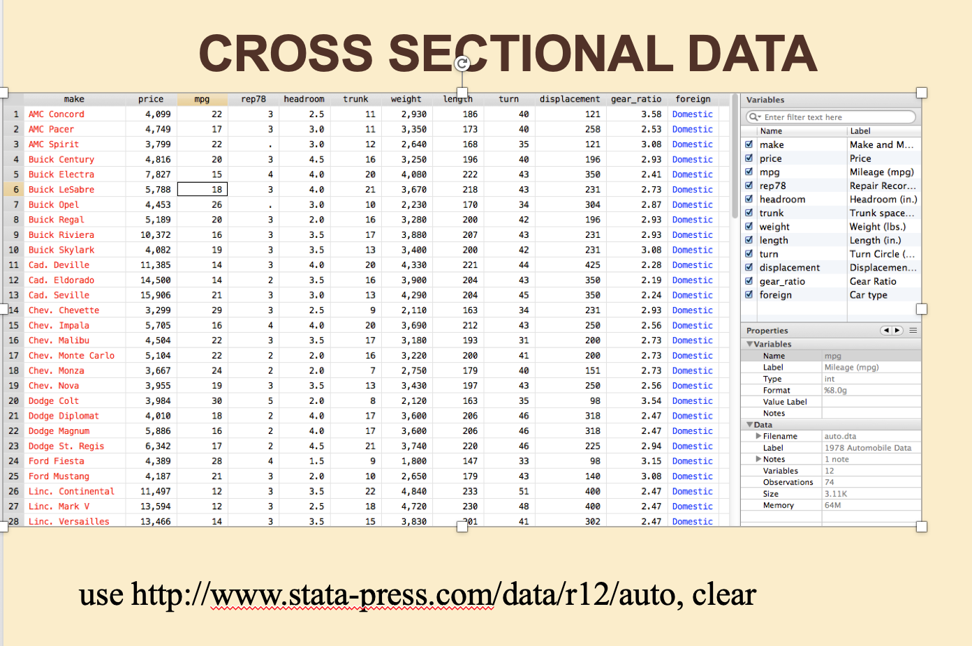
Figure 7.3: Cross-sectional data, viewed in Stata data editor with variable list and properties panes shown
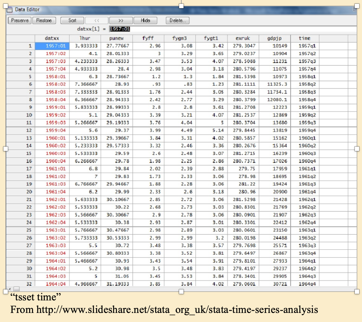
Figure 7.4: Time-series data
Time series: A single ‘unit’ over time… in this case four quarters per year, shown in Stata’s ‘data editor’. (But you shouldn’t usually edit data in this mode – do it with code!)
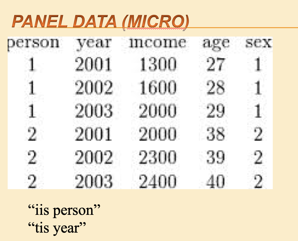
Figure 7.5: Panel data (micro)
xtset is a Stata command to tell Stata you are dealing with panel data. Within this command you specify the variable identifying the unit with iis and the variable identifying the time period with tis.
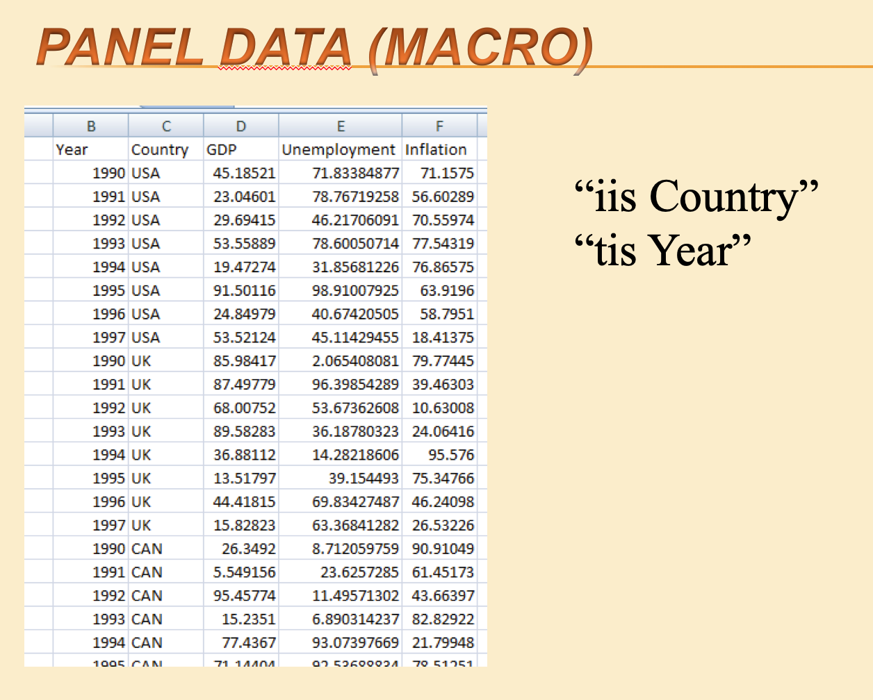
Figure 7.6: Panel data (macro)
Above: Cross-country panel data
String and numeric variables
String variables are text. In their raw form, they usually have quotes (“john smith”,) around them.
Numeric variables can be integers, “floats”, etc, stored in various forms. They are numbers.
Most statistical packages and programming languages treat these two types of variables differently, with a different “syntax” and different commands for each. Be careful.
There are many other data types, with some variation in how these are categorised and stored between languages. E.g.,
‘Factor’ variables (categorical, ordinal)
Logical (true/false)
Date and time variables
7.8 Doing ‘coding’: cleaning, visualizing/summarizing, analysing, and presenting
Some quick important guidelines
Do ALL of your work (cleaning, merging, creating variables, and analysis) by writing code in a ‘script file’ (Stata – a ‘.do file’; R – a ‘.R’ or ‘.Rmd’ file; Python– a ‘.py’ file, I think)
Do your cleaning/construction and analysis in separate files (or at least separate parts of the same file; clean the data first, then analyse it)
Keep this organised and try to write it in a way that you or others, could return to it later.
A good reference… but getting old now: (“Code and Data for the Social Sciences”, 2014, Gentzkow and Shapiro)[https://web.stanford.edu/~gentzkow/research/CodeAndData.pdf]
Some other resources (more up-to-date?) listed Here
7.9 Doing an econometric analysis
Which techniques
You may not be able to use the “ideal” estimation technique; it may be too advanced. But try to be aware (and able to explain) of the strengths and weaknesses of your econometric approach.
Time series, cross section, or panel data?
A major problem is always understanding the difference between a panel and a time series. My students always want to just do a time series regression, and don’t understand why the cross-section dimension is important.”
–University lecturer, Economics
Sections to add:
Common difficulties
Diagnostic tests, etc.
Interpreting your results
The second most frequent issue is that they think they are supposed to get a ‘right’ answer. They stress out when the regression doesn’t come out ‘right’.
– University lecturer, Economics
7.10 Presenting your results
Considering alternative hypotheses and “robustness checks”
Of course it’s OK to use these menu items at first, and to help you find the command you are looking for. When you use the drop-down menu you should also be able see which code it enters into the command window/console, and use that in your own script.↩︎